Blog

  • aws-appsync-react-workshop

    Building real-time applications with React, GraphQL & AWS AppSync

    In this workshop we’ll learn how to build cloud-enabled web applications with React, AppSync, GraphQL, & AWS Amplify.

    Topics we’ll be covering:

    Redeeming the AWS Credit

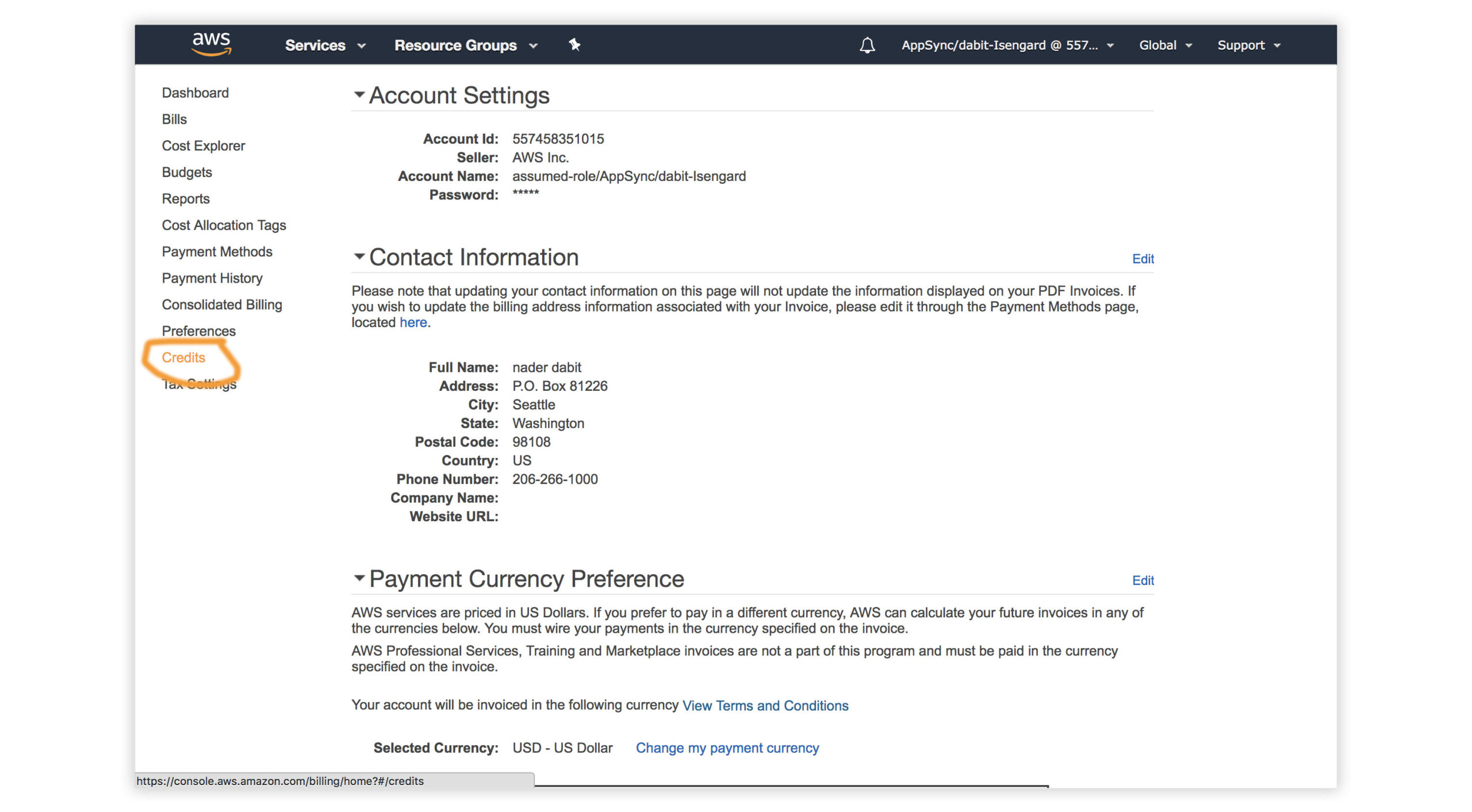
    1. Visit the AWS Console.
    2. In the top right corner, click on My Account.
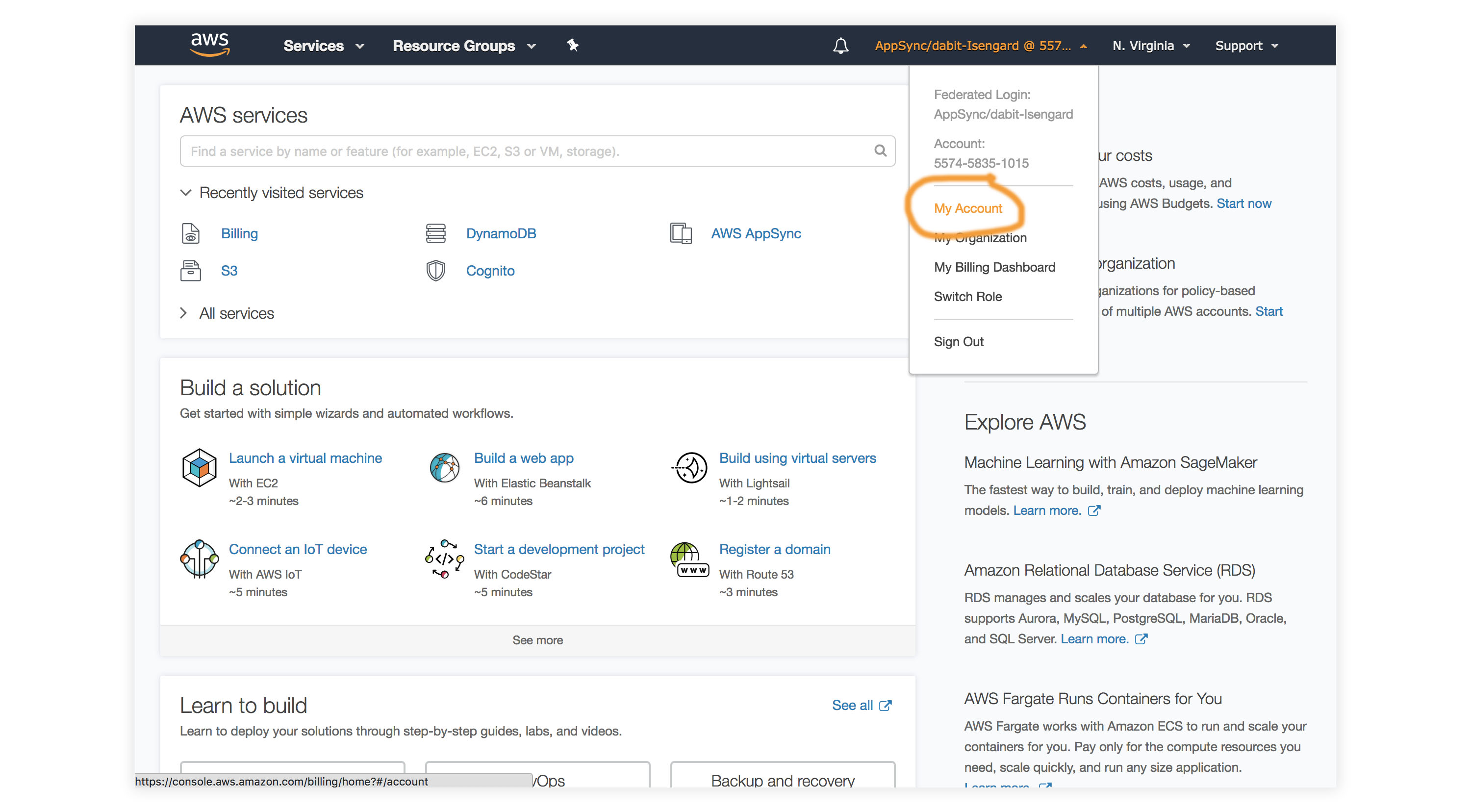
    3. In the left menu, click Credits.

    Getting Started – Creating the React Application

    To get started, we first need to create a new React project using the Create React App CLI.

    $ npx create-react-app my-amplify-app

    Now change into the new app directory & install the AWS Amplify, AWS Amplify React, & uuid libraries:

    $ cd my-amplify-app
    $ npm install --save aws-amplify aws-amplify-react uuid
    # or
    $ yarn add aws-amplify aws-amplify-react uuid

    Installing the CLI & Initializing a new AWS Amplify Project

    Installing the CLI

    Next, we’ll install the AWS Amplify CLI:

    $ npm install -g @aws-amplify/cli

    Now we need to configure the CLI with our credentials:

    $ amplify configure

    If you’d like to see a video walkthrough of this configuration process, click here.

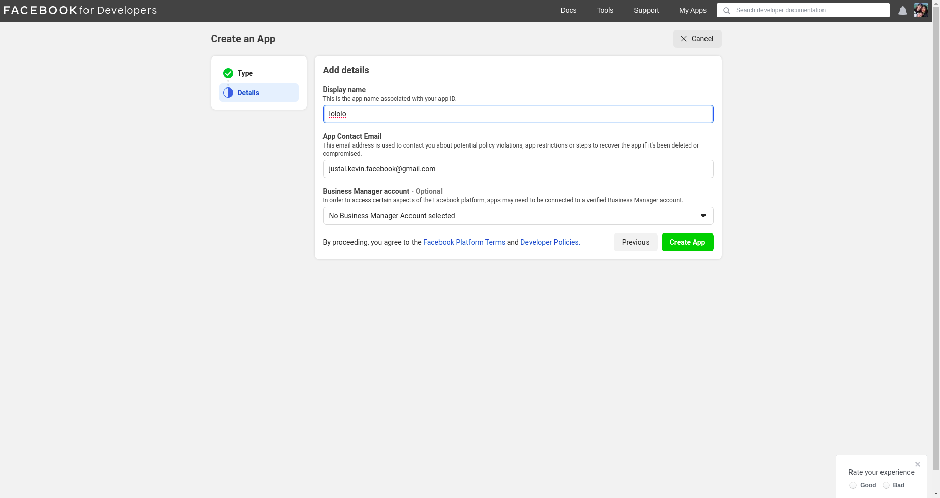
    Here we’ll walk through the amplify configure setup. Once you’ve signed in to the AWS console, continue:

    • Specify the AWS Region: us-east-1 || us-west-2 || eu-central-1
    • Specify the username of the new IAM user: amplify-workshop-user

    In the AWS Console, click Next: Permissions, Next: Tags, Next: Review, & Create User to create the new IAM user. Then, return to the command line & press Enter.

    • Enter the access key of the newly created user:
      ? accessKeyId: (<YOUR_ACCESS_KEY_ID>)
      ? secretAccessKey: (<YOUR_SECRET_ACCESS_KEY>)
    • Profile Name: amplify-workshop-user

    Initializing A New Project

    $ amplify init
    • Enter a name for the project: amplifyreactapp
    • Enter a name for the environment: dev
    • Choose your default editor: Visual Studio Code (or your default editor)
    • Please choose the type of app that you’re building javascript
    • What javascript framework are you using react
    • Source Directory Path: src
    • Distribution Directory Path: build
    • Build Command: npm run-script build
    • Start Command: npm run-script start
    • Do you want to use an AWS profile? Y
    • Please choose the profile you want to use: amplify-workshop-user

    Now, the AWS Amplify CLI has iniatilized a new project & you will see a new folder: amplify & a new file called aws-exports.js in the src directory. These files hold your project configuration.

    To view the status of the amplify project at any time, you can run the Amplify status command:

    $ amplify status

    Configuring the React applicaion

    Now, our resources are created & we can start using them!

    The first thing we need to do is to configure our React application to be aware of our new AWS Amplify project. We can do this by referencing the auto-generated aws-exports.js file that is now in our src folder.

    To configure the app, open src/index.js and add the following code below the last import:

    import Amplify from 'aws-amplify'
    import config from './aws-exports'
    Amplify.configure(config)

    Now, our app is ready to start using our AWS services.

    Adding a GraphQL API

    To add a GraphQL API, we can use the following command:

    $ amplify add api
    
    ? Please select from one of the above mentioned services: GraphQL
    ? Provide API name: ConferenceAPI
    ? Choose an authorization type for the API: API key
    ? Enter a description for the API key: <some description>
    ? After how many days from now the API key should expire (1-365): 365
    ? Do you want to configure advanced settings for the GraphQL API: No
    ? Do you have an annotated GraphQL schema? N 
    ? Do you want a guided schema creation? Y
    ? What best describes your project: Single object with fields
    ? Do you want to edit the schema now? (Y/n) Y

    When prompted, update the schema to the following:

    # amplify/backend/api/ConferenceAPI/schema.graphql
    
    type Talk @model {
      id: ID!
      clientId: ID
      name: String!
      description: String!
      speakerName: String!
      speakerBio: String!
    }

    Local mocking and testing

    To mock and test the API locally, you can run the mock command:

    $ amplify mock api
    
    ? Choose the code generation language target: javascript
    ? Enter the file name pattern of graphql queries, mutations and subscriptions: src/graphql/**/*.js
    ? Do you want to generate/update all possible GraphQL operations - queries, mutations and subscriptions: Y
    ? Enter maximum statement depth [increase from default if your schema is deeply nested]: 2

    This should start an AppSync Mock endpoint:

    AppSync Mock endpoint is running at http://10.219.99.136:20002

    Open the endpoint in the browser to use the GraphiQL Editor.

    From here, we can now test the API.

    Performing mutations from within the local testing environment

    Execute the following mutation to create a new talk in the API:

    mutation createTalk {
      createTalk(input: {
        name: "Full Stack React"
        description: "Using React to build Full Stack Apps with GraphQL"
        speakerName: "Jennifer"
        speakerBio: "Software Engineer"
      }) {
        id name description speakerName speakerBio
      }
    }

    Now, let’s query for the talks:

    query listTalks {
      listTalks {
        items {
          id
          name
          description
          speakerName
          speakerBio
        }
      }
    }

    We can even add search / filter capabilities when querying:

    query listTalksWithFilter {
      listTalks(filter: {
        description: {
          contains: "React"
        }
      }) {
        items {
          id
          name
          description
          speakerName
          speakerBio
        }
      }
    }

    Interacting with the GraphQL API from our client application – Querying for data

    Now that the GraphQL API server is running we can begin interacting with it!

    The first thing we’ll do is perform a query to fetch data from our API.

    To do so, we need to define the query, execute the query, store the data in our state, then list the items in our UI.

    src/App.js

    // src/App.js
    import React from 'react';
    
    // imports from Amplify library
    import { API, graphqlOperation } from 'aws-amplify'
    
    // import query definition
    import { listTalks as ListTalks } from './graphql/queries'
    
    class App extends React.Component {
      // define some state to hold the data returned from the API
      state = {
        talks: []
      }
    
      // execute the query in componentDidMount
      async componentDidMount() {
        try {
          const talkData = await API.graphql(graphqlOperation(ListTalks))
          console.log('talkData:', talkData)
          this.setState({
            talks: talkData.data.listTalks.items
          })
        } catch (err) {
          console.log('error fetching talks...', err)
        }
      }
      render() {
        return (
          <>
            {
              this.state.talks.map((talk, index) => (
                <div key={index}>
                  <h3>{talk.speakerName}</h3>
                  <h5>{talk.name}</h5>
                  <p>{talk.description}</p>
                </div>
              ))
            }
          </>
        )
      }
    }
    
    export default App

    In the above code we are using API.graphql to call the GraphQL API, and then taking the result from that API call and storing the data in our state. This should be the list of talks you created via the GraphiQL editor.

    Feel free to add some styling here to your list if you’d like 😀

    Next, test the app locally:

    $ npm start

    Performing mutations

    Now, let’s look at how we can create mutations.

    To do so, we’ll refactor our initial state in order to also hold our form fields and add an event handler.

    We’ll also be using the API class from amplify again, but now will be passing a second argument to graphqlOperation in order to pass in variables: API.graphql(graphqlOperation(CreateTalk, { input: talk })).

    We also have state to work with the form inputs, for name, description, speakerName, and speakerBio.

    // src/App.js
    import React from 'react';
    
    import { API, graphqlOperation } from 'aws-amplify'
    // import uuid to create a unique client ID
    import uuid from 'uuid/v4'
    
    import { listTalks as ListTalks } from './graphql/queries'
    // import the mutation
    import { createTalk as CreateTalk } from './graphql/mutations'
    
    const CLIENT_ID = uuid()
    
    class App extends React.Component {
      // define some state to hold the data returned from the API
      state = {
        name: '', description: '', speakerName: '', speakerBio: '', talks: []
      }
    
      // execute the query in componentDidMount
      async componentDidMount() {
        try {
          const talkData = await API.graphql(graphqlOperation(ListTalks))
          console.log('talkData:', talkData)
          this.setState({
            talks: talkData.data.listTalks.items
          })
        } catch (err) {
          console.log('error fetching talks...', err)
        }
      }
      createTalk = async() => {
        const { name, description, speakerBio, speakerName } = this.state
        if (name === '' || description === '' || speakerBio === '' || speakerName === '') return
    
        const talk = { name, description, speakerBio, speakerName, clientId: CLIENT_ID }
        const talks = [...this.state.talks, talk]
        this.setState({
          talks, name: '', description: '', speakerName: '', speakerBio: ''
        })
    
        try {
          await API.graphql(graphqlOperation(CreateTalk, { input: talk }))
          console.log('item created!')
        } catch (err) {
          console.log('error creating talk...', err)
        }
      }
      onChange = (event) => {
        this.setState({
          [event.target.name]: event.target.value
        })
      }
      render() {
        return (
          <>
            <input
              name='name'
              onChange={this.onChange}
              value={this.state.name}
              placeholder='name'
            />
            <input
              name='description'
              onChange={this.onChange}
              value={this.state.description}
              placeholder='description'
            />
            <input
              name='speakerName'
              onChange={this.onChange}
              value={this.state.speakerName}
              placeholder='speakerName'
            />
            <input
              name='speakerBio'
              onChange={this.onChange}
              value={this.state.speakerBio}
              placeholder='speakerBio'
            />
            <button onClick={this.createTalk}>Create Talk</button>
            {
              this.state.talks.map((talk, index) => (
                <div key={index}>
                  <h3>{talk.speakerName}</h3>
                  <h5>{talk.name}</h5>
                  <p>{talk.description}</p>
                </div>
              ))
            }
          </>
        )
      }
    }
    
    export default App

    Adding Authentication

    Next, let’s update the app to add authentication.

    To add authentication, we can use the following command:

    $ amplify add auth
    
    ? Do you want to use default authentication and security configuration? Default configuration 
    ? How do you want users to be able to sign in when using your Cognito User Pool? Username
    ? Do you want to configure advanced settings? No, I am done.   

    Using the withAuthenticator component

    To add authentication in the React app, we’ll go into src/App.js and first import the withAuthenticator HOC (Higher Order Component) from aws-amplify-react:

    // src/App.js, import the new component
    import { withAuthenticator } from 'aws-amplify-react'

    Next, we’ll wrap our default export (the App component) with the withAuthenticator HOC:

    // src/App.js, change the default export to this:
    export default withAuthenticator(App, { includeGreetings: true })

    To deploy the authentication service and mock and test the app locally, you can run the mock command:

    $ amplify mock
    
    ? Are you sure you want to continue? Yes

    Next, to test it out in the browser:

    npm start

    Now, we can run the app and see that an Authentication flow has been added in front of our App component. This flow gives users the ability to sign up & sign in.

    Accessing User Data

    We can access the user’s info now that they are signed in by calling Auth.currentAuthenticatedUser() in componentDidMount.

    import {API, graphqlOperation, /* new 👉 */ Auth} from 'aws-amplify'
    
    async componentDidMount() {
      // add this code to componentDidMount
      const user = await Auth.currentAuthenticatedUser()
      console.log('user:', user)
      console.log('user info:', user.signInUserSession.idToken.payload)
    }

    Adding Authorization to the GraphQL API

    Next we need to update the AppSync API to now use the newly created Cognito Authentication service as the authentication type.

    To do so, we’ll reconfigure the API:

    $ amplify update api
    
    ? Please select from one of the below mentioned services: GraphQL   
    ? Choose the default authorization type for the API: Amazon Cognito User Pool
    ? Do you want to configure advanced settings for the GraphQL API: No, I am done

    Next, we’ll test out the API with authentication enabled:

    $ amplify mock

    Now, we can only access the API with a logged in user.

    You’ll notice an auth button in the GraphiQL explorer that will allow you to update the simulated user and their groups.

    Fine Grained access control – Using the @auth directive

    GraphQL Type level authorization with the @auth directive

    For authorization rules, we can start using the @auth directive.

    What if you’d like to have a new Comment type that could only be updated or deleted by the creator of the Comment but can be read by anyone?

    We could add the following type to our GraphQL schema:

    # amplify/backend/api/ConferenceAPI/schema.graphql
    
    type Comment @model @auth(rules: [
      { allow: owner, ownerField: "createdBy", operations: [create, update, delete]},
      { allow: private, operations: [read] }
      ]) {
      id: ID!
      message: String
      createdBy: String
    }

    allow: owner – This allows us to set owner authorization rules.
    allow: private – This allows us to set private authorization rules.

    This would allow us to create comments that only the creator of the Comment could delete, but anyone could read.

    Creating a comment:

    mutation createComment {
      createComment(input:{
        message: "Cool talk"
      }) {
        id
        message
        createdBy
      }
    }

    Listing comments:

    query listComments {
      listComments {
        items {
          id
          message
          createdBy
        }
      }
    }

    Updating a comment:

    mutation updateComment {
      updateComment(input: {
        id: "59d202f8-bfc8-4629-b5c2-bdb8f121444a"
      }) {
        id 
        message
        createdBy
      }
    }

    If you try to update a comment from someone else, you will get an unauthorized error.

    Relationships

    What if we wanted to create a relationship between the Comment and the Talk? That’s pretty easy. We can use the @connection directive:

    # amplify/backend/api/ConferenceAPI/schema.graphql
    
    type Talk @model {
      id: ID!
      clientId: ID
      name: String!
      description: String!
      speakerName: String!
      speakerBio: String!
      comments: [Comment] @connection(name: "TalkComments")
    }
    
    type Comment @model @auth(rules: [
      { allow: owner, ownerField: "createdBy", operations: [create, update, delete]},
      { allow: private, operations: [read] }
      ]) {
      id: ID!
      message: String
      createdBy: String
      talk: Talk @connection(name: "TalkComments")
    }

    Because we’re updating the way our database is configured by adding relationships which requires a global secondary index, we need to delete the old local database:

    $ rm -r amplify/mock-data

    Now, restart the server:

    $ amplify mock

    Now, we can create relationships between talks and comments. Let’s test this out with the following operations:

    mutation createTalk {
      createTalk(input: {
        id: "test-id-talk-1"
        name: "Talk 1"
        description: "Cool talk"
        speakerBio: "Cool gal"
        speakerName: "Jennifer"
      }) {
        id
        name
        description
      }
    }
    
    mutation createComment {
      createComment(input: {
        commentTalkId: "test-id-talk-1"
        message: "Great talk"
      }) {
        id message
      }
    }
    
    query listTalks {
      listTalks {
        items {
          id
          name
          description
          comments {
            items {
              message
              createdBy
            }
          }
        }
      }
    }

    If you’d like to read more about the @auth directive, check out the documentation here.

    Groups

    The last problem we are facing is that anyone signed in can create a new talk. Let’s add authorization that only allows users that are in an Admin group to create and update talks.

    # amplify/backend/api/ConferenceAPI/schema.graphql
    
    type Talk @model @auth(rules: [
      { allow: groups, groups: ["Admin"] },
      { allow: private, operations: [read] }
      ]) {
      id: ID!
      clientId: ID
      name: String!
      description: String!
      speakerName: String!
      speakerBio: String!
      comments: [Comment] @connection(name: "TalkComments")
    }
    
    type Comment @model @auth(rules: [
      { allow: owner, ownerField: "createdBy", operations: [create, update, delete]},
      { allow: private, operations: [read] }
      ]) {
      id: ID!
      message: String
      createdBy: String
      talk: Talk @connection(name: "TalkComments")
    }

    Run the server:

    $ amplify mock

    Click on the auth button and add Admin the user’s groups.

    Now, you’ll notice that only users in the Admin group can create, update, or delete a talk, but anyone can read it.

    Lambda GraphQL Resolvers

    Next, let’s have a look at how to deploy a serverless function and use it as a GraphQL resolver.

    The use case we will work with is fetching data from another HTTP API and returning the response via GraphQL. To do this, we’ll use a serverless function.

    The API we will be working with is the CoinLore API that will allow us to query for cryptocurrency data.

    To get started, we’ll create the new function:

    $ amplify add function
    
    ? Provide a friendly name for your resource to be used as a label for this category in the project: currencyfunction
    ? Provide the AWS Lambda function name: currencyfunction
    ? Choose the function template that you want to use: Hello world function
    ? Do you want to access other resources created in this project from your Lambda function? N
    ? Do you want to edit the local lambda function now? Y

    Update the function with the following code:

    // amplify/backend/function/currencyfunction/src/index.js
    const axios = require('axios')
    
    exports.handler = function (event, _, callback) {
      let apiUrl = `https://api.coinlore.com/api/tickers/?start=1&limit=10`
    
      if (event.arguments) { 
        const { start = 0, limit = 10 } = event.arguments
        apiUrl = `https://api.coinlore.com/api/tickers/?start=${start}&limit=${limit}`
      }
    
      axios.get(apiUrl)
        .then(response => callback(null, response.data.data))
        .catch(err => callback(err))
    }

    In the above function we’ve used the axios library to call another API. In order to use axios, we need be sure that it will be installed by updating the package.json for the new function:

    amplify/backend/function/currencyfunction/src/package.json

    "dependencies": {
      // ...
      "axios": "^0.19.0",
    },

    Next, we’ll update the GraphQL schema to add a new type and query. In amplify/backend/api/ConferenceAPI/schema.graphql, update the schema with the following new types:

    type Coin {
      id: String!
      name: String!
      symbol: String!
      price_usd: String!
    }
    
    type Query {
      getCoins(limit: Int start: Int): [Coin] @function(name: "currencyfunction-${env}")
    }

    Now the schema has been updated and the Lambda function has been created. To test it out, you can run the mock command:

    $ amplify mock

    In the query editor, run the following queries:

    # basic request
    query listCoins {
      getCoins {
        price_usd
        name
        id
        symbol
      }
    }
    
    # request with arguments
    query listCoinsWithArgs {
      getCoins(limit:3 start: 10) {
        price_usd
        name
        id
        symbol
      }
    }

    This query should return an array of cryptocurrency information.

    Deploying the Services

    Next, let’s deploy the AppSync GraphQL API and the Lambda function:

    $ amplify push
    
    ? Do you want to generate code for your newly created GraphQL API? Y
    ? Choose the code generation language target: javascript
    ? Enter the file name pattern of graphql queries, mutations and subscriptions: src/graphql/**/*.js
    ? Do you want to generate/update all possible GraphQL operations - queries, mutations and subscriptions? Y
    ? Enter maximum statement depth [increase from default if your schema is deeply nested] 2

    To view the new AWS AppSync API at any time after its creation, run the following command:

    $ amplify console api

    To view the Cognito User Pool at any time after its creation, run the following command:

    $ amplify console auth

    To test an authenticated API out in the AWS AppSync console, it will ask for you to Login with User Pools. The form will ask you for a ClientId. This ClientId is located in src/aws-exports.js in the aws_user_pools_web_client_id field.

    Hosting via the Amplify Console

    The Amplify Console is a hosting service with continuous integration and continuous deployment.

    The first thing we need to do is create a new GitHub repo for this project. Once we’ve created the repo, we’ll copy the URL for the project to the clipboard & initialize git in our local project:

    $ git init
    
    $ git remote add origin git@github.com:username/project-name.git
    
    $ git add .
    
    $ git commit -m 'initial commit'
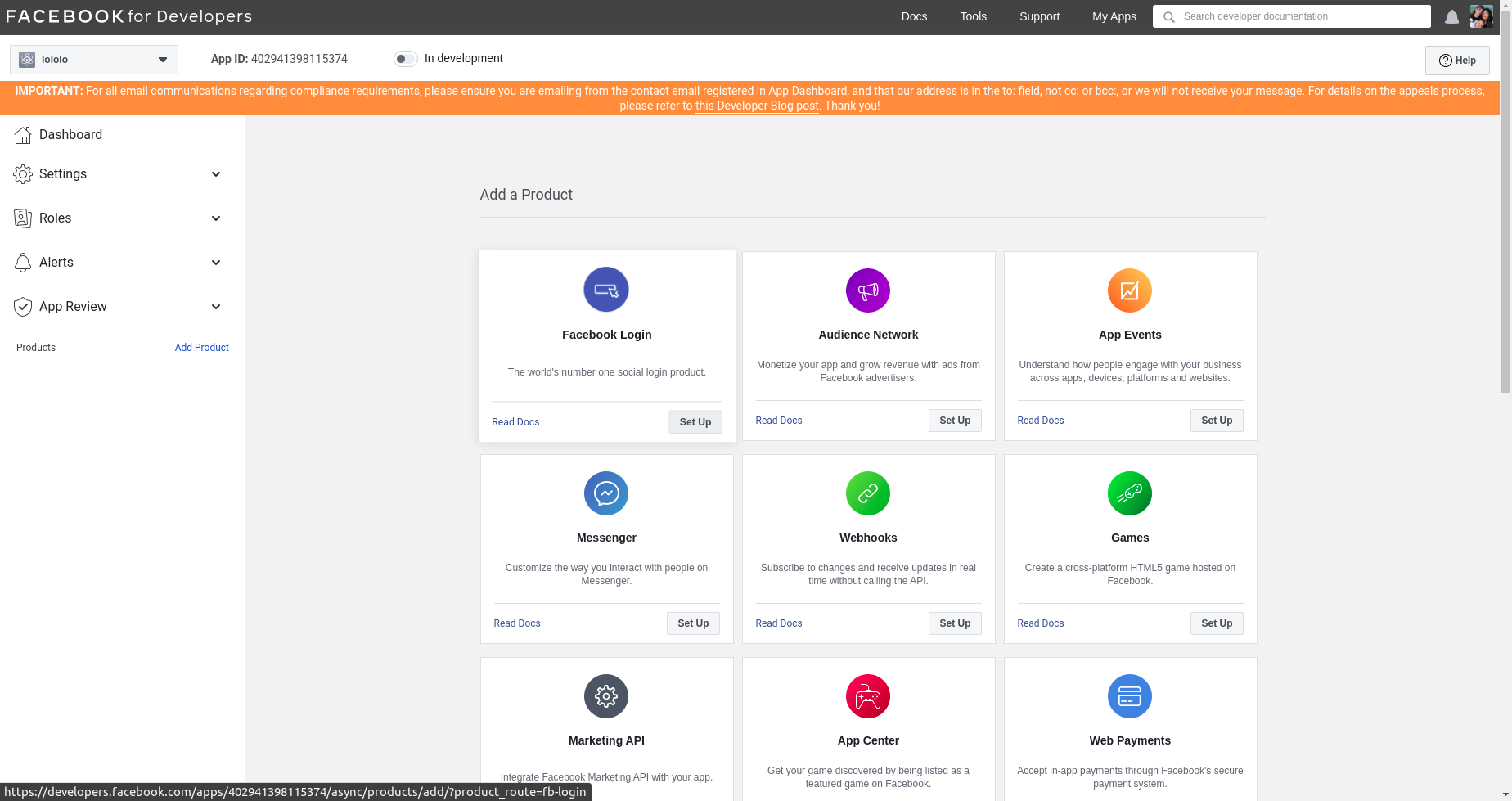
    
    $ git push origin master

    Next we’ll visit the Amplify Console in our AWS account at https://us-east-1.console.aws.amazon.com/amplify/home.

    Here, we’ll click on the app that we deployed earlier.

    Next, under “Frontend environments”, authorize Github as the repository service.

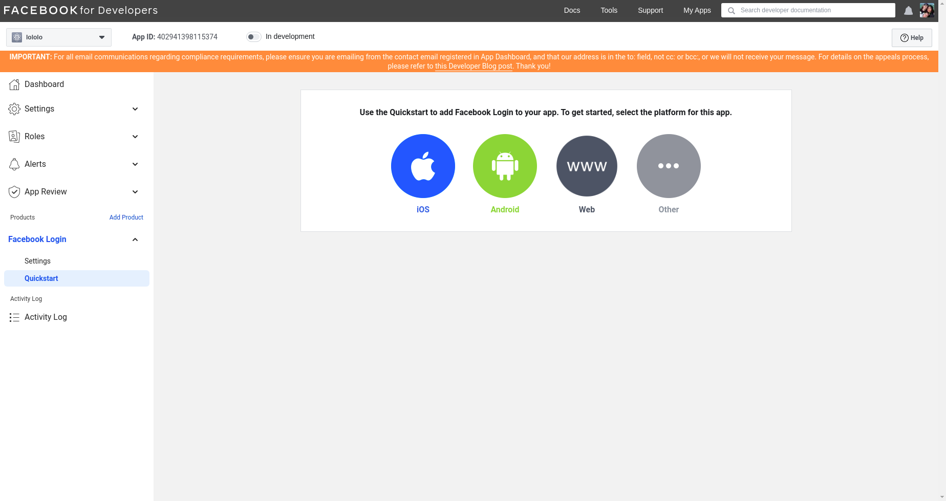
    Next, we’ll choose the new repository & branch for the project we just created & click Next.

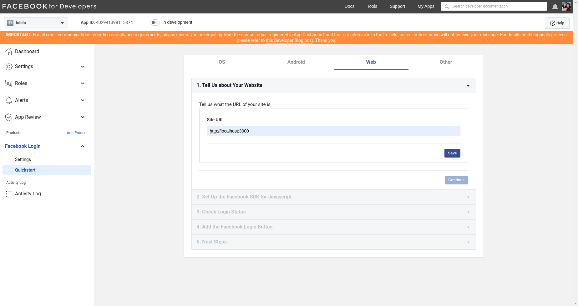
    In the next screen, we’ll create a new role & use this role to allow the Amplify Console to deploy these resources & click Next.

    Finally, we can click Save and Deploy to deploy our application!

    Now, we can push updates to Master to update our application.

    Amplify DataStore

    To implement a GraphQL API with Amplify DataStore, check out the tutorial here

    Removing Services

    If at any time, or at the end of this workshop, you would like to delete a service from your project & your account, you can do this by running the amplify remove command:

    $ amplify remove auth
    
    $ amplify push

    If you are unsure of what services you have enabled at any time, you can run the amplify status command:

    $ amplify status

    amplify status will give you the list of resources that are currently enabled in your app.

    If you’d like to delete the entire project, you can run the delete command:

    $ amplify delete
    Visit original content creator repository
  • aorura

    AORURA

    AORURA LED library, CLI, and emulator.

    Table of contents

    Protocol

    AORURA communicates via a serial connection (19200n8). All commands it supports are exactly two bytes:

    • XX turns the LED off
    • A< puts the LED into its signature shimmering “aurora” state
    • a color byte followed by ! makes the LED light up with the given color
    • a color byte followed by * makes the LED flash with the given color at a half-second interval

    AORURA responds to these commands with a single byte: Y if successful, N if not.

    There’s one more: SS. AORURA responds to this command with two bytes representing the command for its current state.

    AORURA’s initial state is B* (flashing blue).

    Valid color bytes:

    • B: blue
    • G: green
    • O: orange
    • P: purple
    • R: red
    • Y: yellow

    Library

    aorura is a library that implements the AORURA protocol.

    Usage

    Example

    use aorura::*;
    use failure::*;
    
    fn main() -> Fallible<()> {
      let mut led = Led::open("/dev/ttyUSB0")?;
    
      led.set(State::Flash(Color::Red))?;
      led.set(State::Off)?;
    
      assert_eq!(led.get()?, State::Off);
      assert_eq!(State::try_from(b"B*")?, State::Flash(Color::Blue));
    
      Ok(())
    }

    CLI

    aorura-cli is a CLI built on top of the AORURA library.

    Usage

    Usage: aorura-cli <path> [--set STATE]
           aorura-cli --help
    
    Gets/sets the AORURA LED state.
    
    Options:
      --set STATE  set the LED to the given state
    
    States: aurora, flash:COLOR, off, static:COLOR
    Colors: blue, green, orange, purple, red, yellow
    

    Example

    path=/dev/ttyUSB0
    original_state=$(aorura-cli $path)
    
    aorura-cli $path --set flash:yellow
    
    # Do something time-consuming:
    sleep 10
    
    # Revert back to the original LED state:
    aorura-cli $path --set "$original_state"

    Emulator

    aorura-emu is a PTY-based AORURA emulator. It can be used with the library or the CLI in lieu of the hardware.

    Usage

    Usage: aorura-emu <path>
           aorura-emu --help
    
    Emulates AORURA over a PTY symlinked to the given path.
    

    Hardware

    • AORURA-3 (HoloPort and HoloPort+)

      AORURA-3 photo

    • AORURA-UART-1 (HoloPort Nano)

      AORURA-UART-1 photo

    Visit original content creator repository
  • bluerov2_gym

    BlueROV2 Gymnasium Environment

    A Gymnasium environment for simulating and training reinforcement learning agents on the BlueROV2 underwater vehicle. This environment provides a realistic simulation of the BlueROV2’s dynamics and supports various control tasks.

    image

    🌊 Features

    • Realistic Physics: Implements validated hydrodynamic model of the BlueROV2
    • 3D Visualization: Real-time 3D rendering using Meshcat
    • Custom Rewards: Configurable reward functions for different tasks
    • Disturbance Modeling: Includes environmental disturbances for realistic underwater conditions
    • Stable-Baselines3 Compatible: Ready to use with popular RL frameworks
    • Customizable Environment: Easy to modify for different underwater tasks
    • (Future release: spawn multiple AUVs)

    🛠️ Installation

    Prerequisites

    • Python ≥3.10
    • uv (recommended) or pip

    Using uv (Recommended)

    # Clone the repository
    git clone https://github.com/gokulp01/bluerov2_gym.git
    cd bluerov2_gym
    
    # Create and activate a virtual environment
    uv venv
    source .venv/bin/activate  # On Windows: .venv\Scripts\activate
    
    # Install the package
    uv pip install -e .

    Using pip

    # Clone the repository
    git clone https://github.com/gokulp01/bluerov2_gym.git
    cd bluerov2_gym
    
    # Create and activate a virtual environment
    python -m venv .venv
    source .venv/bin/activate  # On Windows: .venv\Scripts\activate
    
    # Install the package
    pip install -e .

    🎮 Usage

    Basic Usage

    import gymnasium as gym
    import bluerov2_gym
    
    # Create the environment
    env = gym.make("BlueRov-v0", render_mode="human")
    
    # Reset the environment
    observation, info = env.reset()
    
    # Run a simple control loop
    while True:
        # Take a random action
        action = env.action_space.sample()
        observation, reward, terminated, truncated, info = env.step(action)
        
        if terminated or truncated:
            observation, info = env.reset()

    Training with Stable-Baselines3 (refer to examples/train.py for full code example)

    from stable_baselines3 import PPO
    from stable_baselines3.common.vec_env import DummyVecEnv, VecNormalize
    
    # Create and wrap the environment
    env = gym.make("BlueRov-v0")
    env = DummyVecEnv([lambda: env])
    env = VecNormalize(env)
    
    # Initialize the agent
    model = PPO("MultiInputPolicy", env, verbose=1)
    
    # Train the agent
    model.learn(total_timesteps=1_000_000)
    
    # Save the trained model
    model.save("bluerov_ppo")

    🎯 Environment Details

    State Space

    The environment uses a Dictionary observation space containing:

    • x, y, z: Position coordinates
    • theta: Yaw angle
    • vx, vy, vz: Linear velocities
    • omega: Angular velocity

    Action Space

    Continuous action space with 4 dimensions:

    • Forward/Backward thrust
    • Left/Right thrust
    • Up/Down thrust
    • Yaw rotation

    Reward Function

    The default reward function considers:

    • Position error from target
    • Velocity penalties
    • Orientation error
    • Custom rewards can be implemented by extending the Reward class

    📊 Examples

    The examples directory contains several scripts demonstrating different uses:

    • test.py: Basic environment testing with manual control and evaluation with trained model
    • train.py: Training script using PPO

    Running Examples

    # Test environment with manual control
    python examples/test.py
    
    # Train an agent
    python examples/train.py

    🖼️ Visualization

    The environment uses Meshcat for 3D visualization. When running with render_mode="human", a web browser window will open automatically showing the simulation. The visualization includes:

    • Water surface effects
    • Underwater environment
    • ROV model
    • Ocean floor with decorative elements (I am no good at this)

    📚 Project Structure

    bluerov2_gym/
    ├── bluerov2_gym/              # Main package directory
    │   ├── assets/               # 3D models and resources
    │   └── envs/                 # Environment implementation
    │       ├── core/            # Core components
    │       │   ├── dynamics.py  # Physics simulation
    │       │   ├── rewards.py   # Reward functions
    │       │   ├── state.py     # State management
    │       │   └── visualization/
    │       │       └── renderer.py  # 3D visualization
    │       └── bluerov_env.py    # Main environment class
    ├── examples/                  # Example scripts
    ├── tests/                    # Test cases
    └── README.md
    

    🔧 Configuration

    The environment can be configured through various parameters:

    • Physics parameters in dynamics.py
    • Reward weights in rewards.py
    • Visualization settings in renderer.py

    📝 Citation

    If you use this environment in your research, please cite:

    @article{puthumanaillam2024tabfieldsmaximumentropyframework,
    title={TAB-Fields: A Maximum Entropy Framework for Mission-Aware Adversarial Planning},
    author={Gokul Puthumanaillam and Jae Hyuk Song and Nurzhan Yesmagambet and Shinkyu Park and Melkior Ornik},
    year={2024},
    eprint={2412.02570},
    archivePrefix={arXiv},
    url={https://arxiv.org/abs/2412.02570} } 
    }

    🤝 Contributing

    Contributions are welcome! Please feel free to submit a Pull Request. For major changes, please open an issue first to discuss what you would like to change.

    1. Fork the repository
    2. Create your feature branch (git checkout -b feature/AmazingFeature)
    3. Commit your changes (git commit -m 'Add some AmazingFeature')
    4. Push to the branch (git push origin feature/AmazingFeature)
    5. Open a Pull Request

    📄 License

    This project is licensed under the MIT License

    🙏 Acknowledgements

    • BlueRobotics for the BlueROV2 specifications
    • OpenAI/Farama Foundation for the Gymnasium framework
    • Meshcat for the visualization library

    📧 Contact

    Gokul Puthumanaillam – @gokulp01 – [gokulp2@illinois.edu]

    Project Link: https://github.com/gokulp01/bluerov2_gym

    Visit original content creator repository

  • torch2coreml

    Convert Torch7 models into Apple CoreML format.

    Short tutorial

    This tool helps convert Torch7 models into Apple CoreML format which can then be run on Apple devices.

    fast-neural-style example app screenshot

    Installation

    pip install -U torch2coreml

    In order to use this tool you need to have these installed:

    • Xcode 9
    • python 2.7

    If you want to run tests, you need MacOS High Sierra 10.13 installed.

    Dependencies

    • coremltools (0.6.2+)
    • PyTorch

    How to use

    Using this library you can implement converter for your own model types. An example of such a converter is located at “example/fast-neural-style/convert-fast-neural-style.py”.
    To implement converters you should use single function “convert” from torch2coreml:

    from torch2coreml import convert

    This function is simple enough to be self-describing:

    def convert(model,
                input_shapes,
                input_names=['input'],
                output_names=['output'],
                mode=None,
                image_input_names=[],
                preprocessing_args={},
                image_output_names=[],
                deprocessing_args={},
                class_labels=None,
                predicted_feature_name='classLabel',
                unknown_layer_converter_fn=None)

    Parameters

    model: Torch7 model (loaded with PyTorch) | str
    A trained Torch7 model loaded in python using PyTorch or path to file
    with model (*.t7).

    input_shapes: list of tuples
    Shapes of the input tensors.

    mode: str (‘classifier’, ‘regressor’ or None)
    Mode of the converted coreml model:
    ‘classifier’, a NeuralNetworkClassifier spec will be constructed.
    ‘regressor’, a NeuralNetworkRegressor spec will be constructed.

    preprocessing_args: dict
    ‘is_bgr’, ‘red_bias’, ‘green_bias’, ‘blue_bias’, ‘gray_bias’,
    ‘image_scale’ keys with the same meaning as
    https://apple.github.io/coremltools/generated/coremltools.models.neural_network.html#coremltools.models.neural_network.NeuralNetworkBuilder.set_pre_processing_parameters

    deprocessing_args: dict
    Same as ‘preprocessing_args’ but for deprocessing.

    class_labels: A string or list of strings.
    As a string it represents the name of the file which contains
    the classification labels (one per line).
    As a list of strings it represents a list of categories that map
    the index of the output of a neural network to labels in a classifier.

    predicted_feature_name: str
    Name of the output feature for the class labels exposed in the Core ML
    model (applies to classifiers only). Defaults to ‘classLabel’

    unknown_layer_converter_fn: function with signature:
    (builder, name, layer, input_names, output_names)
    builder: object – instance of NeuralNetworkBuilder class
    name: str – generated layer name
    layer: object – PyTorch (python) object for corresponding layer
    input_names: list of strings
    output_names: list of strings
    Returns: list of strings for layer output names
    Callback function to handle unknown for torch2coreml layers

    Returns

    model: A coreml model.

    Currently supported

    Models

    Only Torch7 “nn” module is supported now.

    Layers

    List of Torch7 layers that can be converted into their CoreML equivalent:

    1. Sequential
    2. ConcatTable
    3. SpatialConvolution
    4. ELU
    5. ReLU
    6. SpatialBatchNormalization
    7. Identity
    8. CAddTable
    9. SpatialFullConvolution
    10. SpatialSoftMax
    11. SpatialMaxPooling
    12. SpatialAveragePooling
    13. View
    14. Linear
    15. Tanh
    16. MulConstant
    17. SpatialZeroPadding
    18. SpatialReflectionPadding
    19. Narrow
    20. SpatialUpSamplingNearest
    21. SplitTable

    License

    Copyright (c) 2017 Prisma Labs, Inc. All rights reserved.

    Use of this source code is governed by the MIT License that can be found in the LICENSE.txt file.

    Visit original content creator repository

  • Jovian_archive

    Jovian
    A user-friendly Viromics toolkit

    Github release licence Snakemake Version

    For Citations, please use the following DOI:
    Zenodo DOI

    See the documentation:
    Jovian Docs
    Or view an example notebook:
    Launch an example notebook

    IMPORTANT: manuscript is in preparation


    Table of contents


    About Jovian

    Jovian is a Public Health toolkit to automatically process raw NGS data from human clinical matrices (faeces, serum, etc.) into clinically relevant information. It has three main components:

    • Illumina based Metagenomics:
      Includes (amongst other features) data quality control, assembly, taxonomic classification, viral typing, and minority variant identification (quasispecies).
      📝 Please refer to the documentation page for the Illumina Metagenomics workflow for more information.

    • Illumina based Reference-alignment:
      Includes (amongst other features) data quality control, alignment, SNP identification, and consensus-sequence generation.
      ❗ A reference fasta is required.
      📝 Please refer to the documentation page for the Illumina Reference based workflow for more information.

    • Nanopore based Reference-alignment:
      Includes (amongst other features) data quality control, alignment, SNP identification, and consensus-sequence generation.
      ❗ A reference fasta is required.
      ❗ A fasta with primer sequences is required.
      📝 Please refer to the documentation page for the Nanopore Reference based workflow for more information.

    Key features of Jovian:

    • User-friendliness:
      Wetlab personnel can start, configure and interpret results via an interactive web-report. Click here for an example report.
      This makes doing Public Health analyses much more accessible and user-friendly since minimal command-line skills are required.

    • Audit trail:
      All pipeline parameters, software versions, database information and runtime statistics are logged. See details below.

    • Portable:
      Jovian is easily installed on off-site computer systems and at back-up sister institutes. Allowing results to be generated even when the internal grid-computer is down (speaking from experience).


    Commands

    📝 Please see the full Command Line Reference on the documentation site for a more detailed explanation of each command, including example commands for starting an analysis or common usage examples.

    Here, we have a short list of commands and use cases that are used very frequently.

    Use case 1:
    Metagenomic analylsis based on Illumina data:

    bash jovian illumina-metagenomics -i <INPUT DIRECTORY>
    

    Use case 2:
    Align Illumina data against a user-provided reference to generate a consensus genome:

    bash jovian illumina-reference -i <INPUT DIRECTORY> -ref <REFERENCE FASTA>
    

    Use case 3:
    Align Nanopore (multiplex) PCR data against a user-provided reference, remove overrepresented primer sequences, and generate a consensus genome:

    bash jovian nanopore-reference -i <INPUT DIRECTORY> -ref <REFERENCE FASTA> -pr <PRIMER FASTA>
    

    use bash jovian -h to see a full list of commands applicable to the Jovian version that you’re using.


    Features

    📝 Please refer to our documentation for the full list of features

    General features

    • Data quality control and cleaning.
      • Including library fragment length analysis, useful for sample preparation QC.
    • Removal of human* data (patient privacy). *You can use whichever reference you would like. However, Jovian is intended for human clinical samples.
    • Removal of PCR-duplicates for Illumina data.

    Metagenomics specific features

    • Assembly of short reads into bigger scaffolds (often full viral genomes).
    • Taxonomic classification:
      • Every nucleic acid containing biological entity (i.e. not only viruses) is determined up to species level.
      • Lowest Common Ancestor (LCA) analysis is performed to move ambiguous results up to their last common ancestor, which makes results more robust.
    • Viral typing:
      • Several viral families and genera can be taxonomically labelled at the sub-species level as described here.
    • Viral scaffolds are cross-referenced against the Virus-Host interaction database and NCBI host database.
    • Scaffolds are annotated in detail:
      • Depth of coverage.
      • GC content.
      • Open reading frames (ORFs) are predicted.
      • Minority variants (quasispecies) are identified.
    • Importantly, results of all processes listed above are presented via an interactive web-report including an audit trail.

    Reference-alignment specific features

    • All cleaned reads are aligned against the user-provided reference fasta.
    • In the case of Nanopore (multiplex) PCR data, the overrepresented primer sequences are removed.
    • SNPs are called and a consensus genome is generated.
    • Consensus genomes are filtered at the following coverage cut-off thresholds: 1, 5, 10, 30 and 100x.
    • A tabular overview of the breadth of coverage (BoC) at the different coverage cut-off thresholds is generated.
    • Alignments and visualized via IGVjs and allow manual assessment and validation of consensus genomes.

    Visualizations

    All data are visualized via an interactive web-report, as shown here, which includes:

    • A collation of interactive QC graphs via MultiQC.
    • Taxonomic results are presented on three levels:
      • For an entire (multi sample) run, interactive heatmaps are made for non-phage viruses, phages and bacteria. They are stratified to different taxonomic levels.
      • For a sample level overview, Krona interactive taxonomic piecharts are generated.
      • For more detailed analyses, interactive tables are included. Similar to popular spreadsheet applications (e.g. Microsoft Excel).
        • Classified scaffolds
        • Unclassified scaffolds (i.e. “Dark Matter”)
    • Virus typing results are presented via interactive spreadsheet-like tables.
    • An interactive scaffold alignment viewer (IGVjs) is included, containing:
      • Detailed alignment information.
      • Depth of coverage graph.
      • GC content graph.
      • Predicted open reading frames (ORFs).
      • Identified minority variants (quasispecies).
    • All SNP metrics are presented via interactive spreadsheet-like tables, allowing detailed analysis.

    Virus typing

    After a Jovian analysis is finished you can perform virus-typing (i.e. sub-species level taxonomic labelling). These analyses can be started by the command bash jovian -vt [virus keyword], where [virus keyword] can be:

    Keyword Taxon used for scaffold selection Notable virus species
    NoV Caliciviridae Norovirus GI and GII, Sapovirus
    EV Picornaviridae Enteroviruses (Coxsackie, Polio, Rhino, etc.), Parecho, Aichi, Hepatitis A
    RVA Rotavirus A Rotavirus A
    HAV Hepatovirus A Hepatitis A
    HEV Orthohepevirus A Hepatitis E
    PV Papillomaviridae Human Papillomavirus
    Flavi Flaviviridae Dengue (work in progress)
    all All of the above All of the above

    Audit trail

    An audit trail, used for clinical reproducibility and logging, is generated and contains:

    • A unique methodological fingerprint: allowing to exactly reproduce the analysis, even retrospectively by reverting to old versions of the pipeline code.
    • The following information is also logged:
      • Database timestamps
      • (user-specified) Pipeline parameters

    However, it has limitations since several things are out-of-scope for Jovian to control:

    • The virus typing-tools version
      • Currently we depend on a public web-tool hosted by the RIVM. These are developed in close collaboration with – but independently of – Jovian. A versioning system for the virus typing-tools is being worked on, however, this is not trivial and will take some time.
    • Input files and metadata
      • We only save the names and location of input files at the time the analysis was performed. Long-term storage of the data, and documenting their location over time, is the responsibility of the end-user. Likewise, the end-user is responsible for storing datasets with their correct metadata (e.g. clinical information, database versions, etc.). We recommend using iRODS for this as described by Nieroda et al. 2019. While we acknowledge that database versions are vital to replicate results, the databases Jovian uses have no official versioning, hence why we include timestamps only.

    Jovian Illumina Metagenomics workflow visualization Click the image for a full-sized version Jovian Illumina Metagenomics workflow

    Jovian Illumina Reference alignment workflow visualization Click the image for a full-sized version Jovian Illumina Reference workflow

    Jovian Nanopore Reference alignment workflow visualization Click the image for a full-sized version Jovian Nanopore reference workflow

    Requirements

    📝 Please refer to our documentation for a detailed overview of the Jovian requirements here


    Installation

    📝 Please refer to our documentation for detailed instructions regarding the installation of Jovian here

    Usage instructions

    General usage instructions vary for each workflow that we support.
    Please refer to the link below corresponding to the workflow that you wish to use


    FAQ

    Can be found here.


    Example Jovian report

    Can be found here.


    Acknowledgements

    Name Publication Website
    BBtools NA https://jgi.doe.gov/data-and-tools/bbtools/
    BEDtools Quinlan, A.R. and I.M.J.B. Hall, BEDTools: a flexible suite of utilities for comparing genomic features. 2010. 26(6): p. 841-842. https://bedtools.readthedocs.io/en/latest/
    BLAST Altschul, S.F., et al., Gapped BLAST and PSI-BLAST: a new generation of protein database search programs. 1997. 25(17): p. 3389-3402. https://www.ncbi.nlm.nih.gov/books/NBK279690/
    BWA Li, H. (2013). Aligning sequence reads, clone sequences and assembly contigs with BWA-MEM. arXiv preprint arXiv:1303.3997. https://github.com/lh3/bwa
    BioConda Grüning, B., et al., Bioconda: sustainable and comprehensive software distribution for the life sciences. 2018. 15(7): p. 475. https://bioconda.github.io/
    Biopython Cock, P. J., Antao, T., Chang, J. T., Chapman, B. A., Cox, C. J., Dalke, A., … & De Hoon, M. J. (2009). Biopython: freely available Python tools for computational molecular biology and bioinformatics. Bioinformatics, 25(11), 1422-1423. https://biopython.org/
    Bokeh Bokeh Development Team (2018). Bokeh: Python library for interactive visualization. https://bokeh.pydata.org/en/latest/
    Bowtie2 Langmead, B. and S.L.J.N.m. Salzberg, Fast gapped-read alignment with Bowtie 2. 2012. 9(4): p. 357. http://bowtie-bio.sourceforge.net/bowtie2/index.shtml
    Conda NA https://conda.io/
    DRMAA NA http://drmaa-python.github.io/
    FastQC Andrews, S., FastQC: a quality control tool for high throughput sequence data. 2010. https://www.bioinformatics.babraham.ac.uk/projects/fastqc/
    gawk NA https://www.gnu.org/software/gawk/
    GNU Parallel O. Tange (2018): GNU Parallel 2018, March 2018, https://doi.org/10.5281/zenodo.1146014. https://www.gnu.org/software/parallel/
    Git NA https://git-scm.com/
    igvtools NA https://software.broadinstitute.org/software/igv/igvtools
    Jupyter Notebook Kluyver, Thomas, et al. “Jupyter Notebooks-a publishing format for reproducible computational workflows.” ELPUB. 2016. https://jupyter.org/
    Jupyter_contrib_nbextension NA https://github.com/ipython-contrib/jupyter_contrib_nbextensions
    Jupyterthemes NA https://github.com/dunovank/jupyter-themes
    Krona Ondov, B.D., N.H. Bergman, and A.M. Phillippy, Interactive metagenomic visualization in a Web browser. BMC Bioinformatics, 2011. 12: p. 385. https://github.com/marbl/Krona/wiki
    Lofreq Wilm, A., et al., LoFreq: a sequence-quality aware, ultra-sensitive variant caller for uncovering cell-population heterogeneity from high-throughput sequencing datasets. 2012. 40(22): p. 11189-11201. http://csb5.github.io/lofreq/
    MGkit Rubino, F. and Creevey, C.J. 2014. MGkit: Metagenomic Framework For The Study Of Microbial Communities. . Available at: figshare [doi:10.6084/m9.figshare.1269288]. https://bitbucket.org/setsuna80/mgkit/src/develop/
    Minimap2 Li, H., Minimap2: pairwise alignment for nucleotide sequences. Bioinformatics, 2018. https://github.com/lh3/minimap2
    MultiQC Ewels, P., et al., MultiQC: summarize analysis results for multiple tools and samples in a single report. 2016. 32(19): p. 3047-3048. https://multiqc.info/
    Nb_conda NA https://github.com/Anaconda-Platform/nb_conda
    Nb_conda_kernels NA https://github.com/Anaconda-Platform/nb_conda_kernels
    Nginx NA https://www.nginx.com/
    Numpy Walt, S. V. D., Colbert, S. C., & Varoquaux, G. (2011). The NumPy array: a structure for efficient numerical computation. Computing in Science & Engineering, 13(2), 22-30. http://www.numpy.org/
    Pandas McKinney, W. Data structures for statistical computing in python. in Proceedings of the 9th Python in Science Conference. 2010. Austin, TX. https://pandas.pydata.org/
    Picard NA https://broadinstitute.github.io/picard/
    Prodigal Hyatt, D., et al., Prodigal: prokaryotic gene recognition and translation initiation site identification. 2010. 11(1): p. 119. https://github.com/hyattpd/Prodigal/wiki/Introduction
    Python G. van Rossum, Python tutorial, Technical Report CS-R9526, Centrum voor Wiskunde en Informatica (CWI), Amsterdam, May 1995. https://www.python.org/
    Qgrid NA https://github.com/quantopian/qgrid
    SAMtools Li, H., et al., The sequence alignment/map format and SAMtools. 2009. 25(16): p. 2078-2079. http://www.htslib.org/
    SPAdes Nurk, S., et al., metaSPAdes: a new versatile metagenomic assembler. Genome Res, 2017. 27(5): p. 824-834. http://cab.spbu.ru/software/spades/
    seqkit Shen, Wei, et al. “SeqKit: a cross-platform and ultrafast toolkit for FASTA/Q file manipulation.” PloS one 11.10 (2016). https://github.com/shenwei356/seqkit
    Seqtk NA https://github.com/lh3/seqtk
    Snakemake Köster, J. and S.J.B. Rahmann, Snakemake—a scalable bioinformatics workflow engine. 2012. 28(19): p. 2520-2522. https://snakemake.readthedocs.io/en/stable/
    Tabix NA www.htslib.org/doc/tabix.html
    tree NA http://mama.indstate.edu/users/ice/tree/
    Trimmomatic Bolger, A.M., M. Lohse, and B. Usadel, Trimmomatic: a flexible trimmer for Illumina sequence data. Bioinformatics, 2014. 30(15): p. 2114-20. www.usadellab.org/cms/?page=trimmomatic
    Virus-Host Database Mihara, T., Nishimura, Y., Shimizu, Y., Nishiyama, H., Yoshikawa, G., Uehara, H., … & Ogata, H. (2016). Linking virus genomes with host taxonomy. Viruses, 8(3), 66. http://www.genome.jp/virushostdb/note.html
    Virus typing tools Kroneman, A., Vennema, H., Deforche, K., Avoort, H. V. D., Penaranda, S., Oberste, M. S., … & Koopmans, M. (2011). An automated genotyping tool for enteroviruses and noroviruses. Journal of Clinical Virology, 51(2), 121-125. https://www.ncbi.nlm.nih.gov/pubmed/21514213

    Authors

    • Dennis Schmitz (RIVM and EMC)
    • Sam Nooij (RIVM and EMC)
    • Robert Verhagen (RIVM)
    • Thierry Janssens (RIVM)
    • Jeroen Cremer (RIVM)
    • Florian Zwagemaker (RIVM)
    • Mark Kroon (RIVM)
    • Erwin van Wieringen (RIVM)
    • Harry Vennema (RIVM)
    • Annelies Kroneman (RIVM)
    • Marion Koopmans (EMC)

    This project/research has received funding from the European Union’s Horizon 2020 research and innovation programme under grant agreement No. 643476. and the Dutch working group on molecular diagnostics (WMDI).


    Visit original content creator repository
  • SLID-on-Microcontrollers

    SLID on a microcontroller

    For the ETHZ course of Machine Learning on Microcontrollers we had to come up with a project idea that uses a neural network which can run on a STM32 UC with limited resources (64kB RAM, 1 Core running at 80MHz). We decided to use the onboard microphone and detect spoken languages in real-time.

    Project Overview

    Signal Processing and Feature Extraction

    The onboard microphone samples the audio at about 8kHz which was found to be enough, since human speech is mainly in region of 200Hz-4kHz. But even at 8kHz the RAM is filled very fast. Hence, we calculated MFCC features every 256 samples with an overlap of 50%. 12 mel-bins are used, and we aggregated 625 frames before making inference, which is about 10 seconds of speech. image Since this needs to be done in real-time, CMSID-DSP was used which can calculate the MFCC features in Q15 very fast. It has a python wrapper which we used to train the network on the right features already, because they differ a lot from librosa or pytorch implementations! The model was trained using keras and converted to a fully quantized int8 network with tensorflow-lite. This reduced the weight size from 2523 kB to 651 kB while the accuracy only decreased by 0.03%.

    Convolutional Neural Network

    We used a simple CNN, because the network weights need to fit on the ram during inference. The dataset was the Kaggle SLID dataset, where we had several papers as a baseline. image

    Model comparison

    We wanted to compare our model accuracy with other model types and implementations from other papers. In the following table one can see different important factors, such as Flash and RAM needed, which is our main constraint. Luckily our model performed extremely well on the dataset despite its small size while having an inference time of about 4 seconds. image

    Prerequisites

    The project was developed on Windows 10. You will need CubeIDE with the Ai Extension. To easily compile the cmsis-dsp library Ubuntu on WSL2 is used and python and anaconda is installed on the subsystem instead on Windows. All python scripts are run on WSL!

    The platform is an STM32L475.

    Installation

    • clone the repository

    From here run all commands on the Ubuntu subsystem:

    • create a new python environment on WSL using e.g. conda conda create -n slid python=3.8 and activate it conda activate slid
    • install the requirements pip install -r requirements.txt
    • download the dataset kaggle datasets download -d toponowicz/spoken-language-identification
    • extract the dataset and copy the train and test folder to the folder audio_processing
    • from the project root folder run python3 audio_processing/generate_dataset.py (this takes some time)

    Now you will find a folder names as cmsis_[sample_rate]_[num_mel_bins]_[num_mel_windows] that contains the converted mel spectograms as npz files.

    Train the network

    In the model foder you can find the config file. If you want to track training using WANDB you can put in your API key there. The root entry should be the name of the just created dataset with the npz files.

    Start the training from the project root directory with python3 models/train.py

    Once the model has been trained it will be saved as h5 file. Quantize the network with python3 models/tinify.py. This will generate a tflite model.

    Deploy

    Start CubeIDE with the CUBE-AI plugin and load the project from the CubeIDE folder. If it doesn’t work try downloading an older version. Once the upload is done, connect to the STM via serial and press the onboard button to start recording.

    This part is the most complicated as CUBE-AI seems to have its bad days often. Probably it is better to generate a new project from scratch and convert the settings and code to your version.

    Visit original content creator repository
  • LABORATORY-PASSPORT

    LABORATORY-PASSPORT

    I discover few weeks ago the library Passport.js that you can find at this URL : http://www.passportjs.org/

    It makes multiple Authentication through google, facebook, twitter and so on easy using just the ClientId and ClientSecret of the different platform.

    It becomes a must have in my toolbox for managing this kind of challenge.

    Plan

    1. How to use Passport.js
    2. How to create clientID and clientSecret for facebook
    3. How to create clientID and clientSecret for google

    How to use Passport.js

    1. Install Passport.js
    $ npm install Passport.js
    

    In the Express server, use :

    const passport = require('passport');
    
    app.use(passport.initialize());
    app.use(passport.session());
    
    passport.serializeUser(function (user, cb) {
      cb(null, user);
    });
    
    passport.deserializeUser(function (obj, cb) {
      cb(null, obj);
    });
    
    1. Install the dependencies depending of the passport we need

    facebook

    $ npm install passport-facebook
    

    google

    $ npm install passport-google-oauth
    
    1. Enable the Passport depending of the passport

    facebook

    const FacebookStrategy = require('passport-facebook').Strategy;
    
    passport.use(new FacebookStrategy({
        clientID: config.facebookAuth.clientID,
        clientSecret: config.facebookAuth.clientSecret,
        callbackURL: config.facebookAuth.callbackURL
      }, function (accessToken, refreshToken, profile, done) {
        return done(null, profile);
      }
    ));
    

    google

    const GoogleStrategy = require('passport-google-oauth').OAuth2Strategy;
    
    passport.use(new GoogleStrategy({
        clientID: config.googleAuth.clientID,
        clientSecret: config.googleAuth.clientSecret,
        callbackURL: config.googleAuth.callbackURL
      }, function (accessToken, refreshToken, profile, done) {
        return done(null, profile);
      }
    ));
    
    1. Add the ClientID and ClientSecret inside the config.js (see below how to get them)

    2. Create the route for getting the information out of the Authentication

    The scope depend of the Strategy (facebook or google…) and can be find on the documentation of the strategy (google documentation or facebook documentation…)

    facebook

    router.get('/profile', isLoggedIn, function (req, res) {
      console.log(req.user)
    });
    
    router.get('/auth/facebook', passport.authenticate('facebook', {
      scope: ['public_profile', 'email']
    }));
    
    router.get('/auth/facebook/callback',
      passport.authenticate('facebook', {
        successRedirect: '/profile',
        failureRedirect: '/error'
      })
    );
    

    google

    router.get('/profile_google', isLoggedIn, function (req, res) {
      console.log(req.user)
    });
    
    router.get('/auth/google', passport.authenticate('google', {
      scope: ['profile', 'email']
    }));
    
    router.get('/auth/google/callback',
      passport.authenticate('google', {
        successRedirect: '/profile_google',
        failureRedirect: '/error'
      })
    );
    

    How to create clientID and clientSecret for facebook

    1. First, connect to the facebook developer console : https://developers.facebook.com/

    Alt text

    1. Click on create a new app and choose the type of app (none in my case)

    Alt text

    1. Add the name to display in the facebook developer interface

    Alt text

    1. Click on facebook login

    Alt text

    1. Click on www since we will be building a website

    Alt text

    1. Since we will be testing in it locally, we will enter the website : http://localhost:3000/

    Alt text

    1. We then arrive on a page where we can find the ClientId (App ID) and the ClientSecret (App Secret) to enter in our config.js file

    Alt text

    How to create clientID and clientSecret for google

    1. First, connect to the google console : https://console.cloud.google.com/

    Alt text

    1. Search in the bar on the top oauth and click on identifiants

    Alt text

    1. Once the page loaded, click on the top create identifiants

    Alt text

    1. In the dropdown, click on ID Client OAuth

    Alt text

    1. Choose the type of application (web application in this case), add a name and dont forget to add the redirection URI at the bottom. Since I am working locally, it will be : http://localhost:3000

    Alt text

    1. You then will get a popup with the ClientID and ClientSecret that you can copy and paste into the config.js file.

    Alt text

    Visit original content creator repository
  • basquete

    Atividade Prática Supervisionada – Lógica de Programação

    Dados Estatísticos – Time de Basquete

    Supervisionado por: Simone de Abreu e Igor Oliveira Borges

    Descrição da Atividade

    A ideia da atividade é fazer um programa que implemente um relatório estatístico dos jogadores de um time de basquete de uma temporada. Esse relatório é importante para o técnico definir se seu time está com índices de desenvolvimento bons em relação aos demais times da temporada.

    Sabe-se que em um time de basquete são necessários 5 jogadores em quadra, podendo ter até outros 5 jogadores reservas, contabilizando 10 jogadores por time no total.

    Para cada um dos jogadores do time, seu programa deve ler o nome e a altura. Usar um vetor de Strings para armazenar os nomes e um vetor para armazenar as alturas.

    Após a entrada dos dados dos 10 jogadores, o programa deve apresentar o seguinte menu de opções:

    ======== TIME DE BASQUETE ========
    1 – Dados dos jogadores
    2 – Média de alturas
    3 – Desvio padrão das alturas
    4 – Maior e Menor altura
    5 – Mediana das alturas
    6 – Finalizar
    
    Digite uma opção:
    

    Itens do Menu

    1. Exibir o nome e a altura de cada jogador do time.
    2. Calcular e apresentar a média das alturas do time de basquete.
    3. Apenas se a média já estiver sido calculada, calcular o desvio padrão
      que é dado pela fórmula: (Σ(alturasˆ2) + total de alturas) - mediaˆ2.
    4. Encontrar o jogador mais alto e o jogador mais baixo do time. Apresentar o nome do jogador e a sua altura.
    5. Calcula a mediana das alturas. A mediana é o elemento central de uma lista ordenada. Caso o conjunto de dados seja par, então a mediana é a média dos dois valores centrais. Pesquise como “ordenar vetor em JAVA”.
      Lembre-se que o vetor de nomes também devem ser alterados, para tanto, pesquise a função de cópia de strings – clone().
    6. Finaliza a execução do programa.

    Regras e Restrições

    ara o correto desenvolvimento do programa algumas regras e restrições devem ser cumpridas:

    1. A tela de início do programa deve apresentar (System.out.println()) o nome completo e o RA de cada integrante do grupo!
    2. A altura de cada jogador, não pode ser 0 negativa. Caso seja digitado um valor inválido, o programa deverá solicitar um novo valor.
    3. Para qualquer uma das regras listadas, o programa não pode ser finalizado. O programa deve fazer as validações de entrada e somente prosseguir quando os dados de entrada forem válidos.
    4. O programa somente deve ser finalizado ao escolher o item 6 do menu.
    5. Pode utilizar o conceito de métodos – pesquisar nos livros de referência.
    6. Para armazenar os nomes dos jogadores, o grupo deve pesquisar o
      conceito de matrizes (“vetor de Strings em Java” no google).

    Entregáveis

    O trabalho deve ser desenvolvido em equipes de no mínimo 3 e no máximo 5 alunos.
    Cada equipe deve realizar a entrega do projeto compactado, no formato ZIP, pelo Blackboard.

    Critérios de Avaliação

    Cada grupo terá o seu trabalho avaliado utilizando os seguintes critérios:

    • Correta implementação e funcionamento do algoritmo.
    • Legibilidade (comentários e organização).
    • Nomeação adequada de variáveis.
    • Pontualidade na entrega no Blackboard.

    Visit original content creator repository