In this project, you will create an app with multiple flavors that uses
multiple libraries and Google Cloud Endpoints. The finished app will consist
of four modules. A Java library that provides jokes, a Google Cloud Endpoints
(GCE) project that serves those jokes, an Android Library containing an
activity for displaying jokes, and an Android app that fetches jokes from the
GCE module and passes them to the Android Library for display.
Why this Project
As Android projects grow in complexity, it becomes necessary to customize the
behavior of the Gradle build tool, allowing automation of repetitive tasks.
Particularly, factoring functionality into libraries and creating product
flavors allow for much bigger projects with minimal added complexity.
What Will I Learn?
You will learn the role of Gradle in building Android Apps and how to use
Gradle to manage apps of increasing complexity. You’ll learn to:
Add free and paid flavors to an app, and set up your build to share code between them
Factor reusable functionality into a Java library
Factor reusable Android functionality into an Android library
Configure a multi project build to compile your libraries and app
Use the Gradle App Engine plugin to deploy a backend
Configure an integration test suite that runs against the local App Engine development server
Video
I’ve created a video demonstrating the app. Click here to view the video on YouTube.
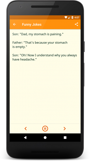
This is the starting point for the final project, which is provided to you in
the course repository. It
contains an activity with a banner ad and a button that purports to tell a
joke, but actually just complains. The banner ad was set up following the
instructions here:
You may need to download the Google Repository from the Extras section of the
Android SDK Manager.
You will also notice a folder called backend in the starter code.
It will be used in step 3 below, and you do not need to worry about it for now.
When you can build an deploy this starter code to an emulator, you’re ready to
move on.
Step 1: Create a Java library
Your first task is to create a Java library that provides jokes. Create a new
Gradle Java project either using the Android Studio wizard, or by hand. Then
introduce a project dependency between your app and the new Java Library. If
you need review, check out demo 4.01 from the course code.
Make the button display a toast showing a joke retrieved from your Java joke
telling library.
Step 2: Create an Android Library
Create an Android Library containing an Activity that will display a joke
passed to it as an intent extra. Wire up project dependencies so that the
button can now pass the joke from the Java Library to the Android Library.
For review on how to create an Android library, check out demo 4.03. For a
refresher on intent extras, check out;
This next task will be pretty tricky. Instead of pulling jokes directly from
our Java library, we’ll set up a Google Cloud Endpoints development server,
and pull our jokes from there. The starter code already includes the GCE module
in the folder called backend.
Before going ahead you will need to be able to run a local instance of the GCE
server. In order to do that you will have to install the Cloud SDK:
Note: You do not need to follow the rest of steps in the migration guide, only
the Setup Cloud SDK.
Start or stop your local server by using the gradle tasks as shown in the following
screenshot:
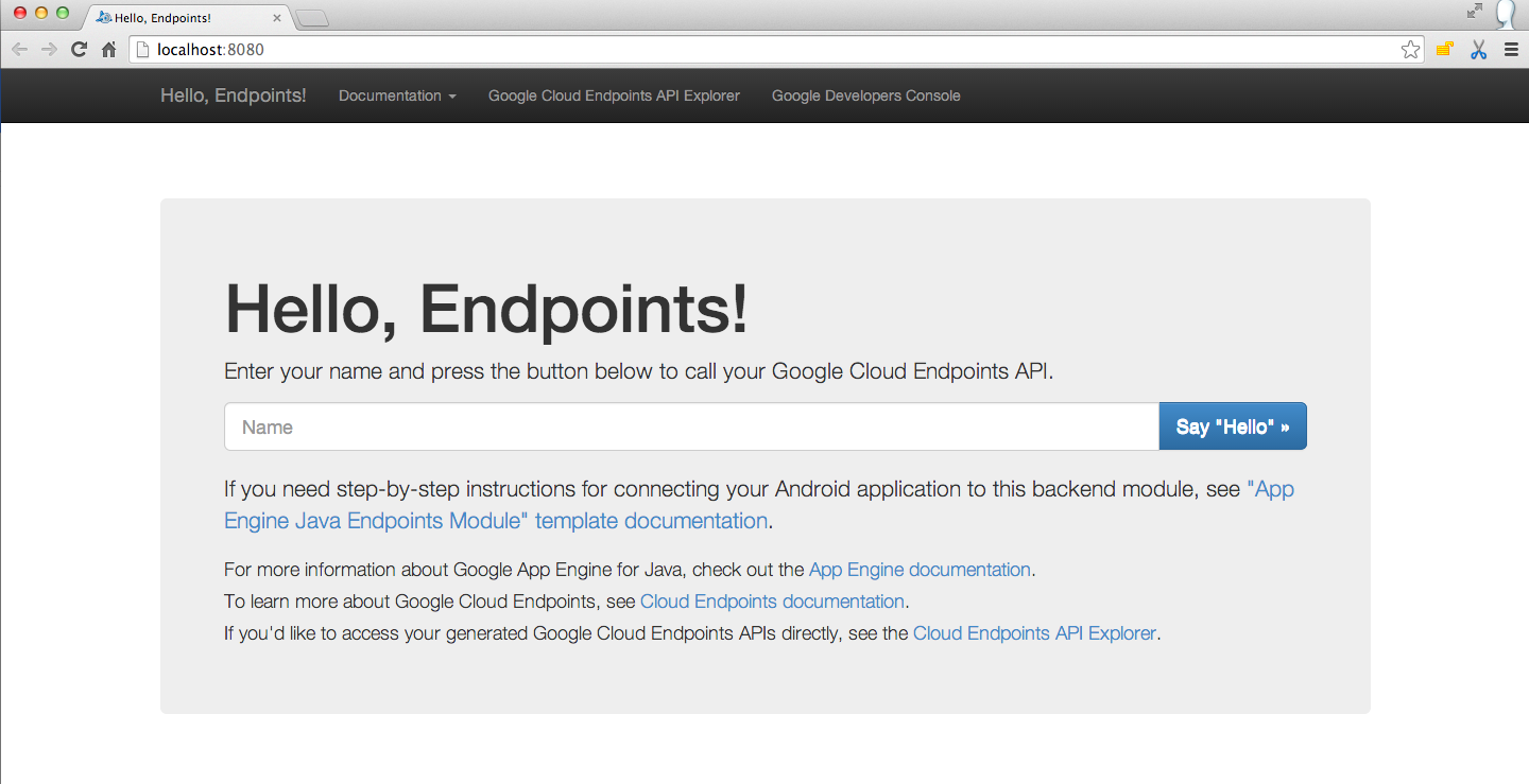
Once your local GCE server is started you should see the following at
localhost:8080
Now you are ready to continue!
Introduce a project dependency between your Java library
and your GCE module, and modify the GCE starter code to pull jokes from your Java library.
Create an AsyncTask to retrieve jokes using the template included int these
instructions.
Make the button kick off a task to retrieve a joke,
then launch the activity from your Android Library to display it.
Step 4: Add Functional Tests
Add code to test that your Async task successfully retrieves a non-empty
string. For a refresher on setting up Android tests, check out demo 4.09.
Step 5: Add a Paid Flavor
Add free and paid product flavors to your app. Remove the ad (and any
dependencies you can) from the paid flavor.
Optional Tasks
For extra practice to make your project stand out, complete the following tasks.
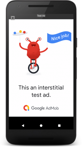
Add Interstitial Ad
Follow these instructions to add an interstitial ad to the free version.
Display the ad after the user hits the button, but before the joke is shown.
Add a loading indicator that is shown while the joke is being retrieved and
disappears when the joke is ready. The following tutorial is a good place to
start:
GitHub’s Watch feature doesn’t send notifications when commits are pushed.
This script aims to implement this feature and much more.
Call for maintainers: I don’t use this project myself anymore but IFTTT
instead (see below). If you’re interested in taking over the maintenance of
this project, or just helping, please let me know (e.g. by opening an issue).
That’s it. As long as your machine is running you’ll get e-mails when something gets pushed on a repo you’re watching.
NOTES:
The e-mails are likely to be considered as spam until you mark one as
non-spam in your e-mail client. Or use the --mailfrom option.
If you’re watching 15 repos or more, you probably want to use the --credentials option to make sure you don’t hit the GitHub API rate limit.
Other/Advanced usage
gicowa is a generic command-line tool with which you can make much more that
just implementing the use case depicted in the introduction. This section
shows what it can.
$ gicowa lastrepocommits AurelienLourot/github-commit-watcher since 2015 07 05 09 12 00
lastrepocommits AurelienLourot/github-commit-watcher since 2015-07-05 09:12:00
Last commit pushed on 2015-07-05 10:48:58
Committed on 2015-07-05 10:46:27 - Aurelien Lourot - Minor cleanup.
Committed on 2015-07-05 09:39:01 - Aurelien Lourot - watchlist command implemented.
Committed on 2015-07-05 09:12:00 - Aurelien Lourot - argparse added.
NOTES:
Keep in mind that a commit’s committer timestamp isn’t the time at
which it gets pushed.
The lines starting with Committed on list commits on the master
branch only. Their timestamps are the committer timestamps.
The line starting with Last commit pushed on shows the time at which a
commit got pushed on the repository for the last time on any branch.
List last commits on repos watched by a user
$ gicowa lastwatchedcommits AurelienLourot since 2015 07 04 00 00 00
lastwatchedcommits AurelienLourot since 2015-07-04 00:00:00
AurelienLourot/crouton-emacs-conf - Last commit pushed on 2015-07-04 17:10:18
AurelienLourot/crouton-emacs-conf - Committed on 2015-07-04 17:08:48 - Aurelien Lourot - Support for Del key.
brillout/FasterWeb - Last commit pushed on 2015-07-04 16:40:54
brillout/FasterWeb - Committed on 2015-07-04 16:38:55 - brillout - add README
AurelienLourot/github-commit-watcher - Last commit pushed on 2015-07-05 10:48:58
AurelienLourot/github-commit-watcher - Committed on 2015-07-05 10:46:27 - Aurelien Lourot - Minor cleanup.
AurelienLourot/github-commit-watcher - Committed on 2015-07-05 09:39:01 - Aurelien Lourot - watchlist command implemented.
AurelienLourot/github-commit-watcher - Committed on 2015-07-05 09:12:00 - Aurelien Lourot - argparse added.
AurelienLourot/github-commit-watcher - Committed on 2015-07-05 09:07:14 - AurelienLourot - Initial commit
NOTE: if you’re watching 15 repos or more, you probably want to use the --credentials option to make sure you don’t hit the GitHub API rate limit.
List last commits since last run
Any listing command taking a since <timestamp> argument takes also a sincelast one. It will then use the time where that same command has been
run for the last time on that machine with the option --persist. This option
makes gicowa remember the last execution time of each command in ~/.gicowa.
$ git clone https://github.com/quick-trade/quick_trade.git
$ pip3 install -r quick_trade/requirements.txt
$ cd quick_trade
$ python3 setup.py install
$ cd ..
Customize your strategy!
fromquick_trade.plotsimportTraderGraph, make_trader_figureimportccxtfromquick_tradeimportstrategy, TradingClient, Traderfromquick_trade.utilsimportTradeSideclassMyTrader(qtr.Trader):
@strategydefstrategy_sell_and_hold(self):
ret= []
foriinself.df['Close'].values:
ret.append(TradeSide.SELL)
self.returns=retself.set_credit_leverages(2) # if you want to use a leverageself.set_open_stop_and_take(stop)
# or... set a stop loss with only one line of codereturnretclient=TradingClient(ccxt.binance())
df=client.get_data_historical("BTC/USDT")
trader=MyTrader("BTC/USDT", df=df)
trader.connect_graph(TraderGraph(make_trader_figure()))
trader.set_client(client)
trader.strategy_sell_and_hold()
trader.backtest()
正式英文:
C#, pronounced “C Sharp,” is a modern, object-oriented programming language developed by Microsoft that runs on the .NET framework.
西班牙文:
C#, pronunciado “C Sharp”, es un lenguaje de programación moderno y orientado a objetos desarrollado por Microsoft que se ejecuta en el marco .NET.
关于该主题的数学研究:
在计算机科学中,编程语言的设计和实现涉及形式语言和自动机理论等数学领域。C# 的类型系统、内存管理和并发模型等特性可以通过数学模型进行分析和验证,以确保语言的可靠性和安全性。例如,类型系统可以使用类型理论来证明程序的正确性,而并发模型可以通过 Petri 网等工具进行建模和分析。
C#(发音为 "C Sharp")是由微软开发的现代、面向对象的编程语言,运行在 .NET 框架上。
**中文**:
C#(发音为 "C Sharp")是由微软开发的现代、面向对象的编程语言,运行在 .NET 框架上。
**正式英文**:
C#, pronounced "C Sharp," is a modern, object-oriented programming language developed by Microsoft that runs on the .NET framework.
**西班牙文**:
C#, pronunciado "C Sharp", es un lenguaje de programación moderno y orientado a objetos desarrollado por Microsoft que se ejecuta en el marco .NET.
**文言文**:
C#,读作 "C Sharp",乃微软所开发之现代面向对象编程语言,运行于 .NET 框架上。
**Prolog**:
```prologlanguage(csharp).developer(microsoft).paradigm(object_oriented).framework(dotnet).
关于该主题的数学研究:
在计算机科学中,编程语言的设计和实现涉及形式语言和自动机理论等数学领域。C# 的类型系统、内存管理和并发模型等特性可以通过数学模型进行分析和验证,以确保语言的可靠性和安全性。例如,类型系统可以使用类型理论来证明程序的正确性,而并发模型可以通过 Petri 网等工具进行建模和分析。
Premature optimization is a term that refers to the practice of attempting to improve the efficiency of a program or system too early in the development process, before understanding if or where optimization is actually needed. This approach can often lead to increased complexity, more difficult code maintenance, and can even introduce bugs, all without a guaranteed benefit to performance.
Here’s a breakdown of why premature optimization is often discouraged and how to approach it wisely:
1. The Risks of Premature Optimization
Increased Complexity: Attempting to optimize early can make the codebase more complex, often involving non-intuitive, “clever” code that’s harder to understand and maintain.
Reduced Flexibility: Early optimizations often “lock in” specific design choices, making it difficult to adapt the code later on if requirements change.
Wasted Resources: Optimizing parts of the program that don’t significantly impact overall performance can waste development time and effort. It’s common for only a small percentage of code to impact runtime, so optimizing other parts yields little benefit.
Bug Introduction: Optimized code can introduce subtle bugs, particularly if the code sacrifices clarity for performance.
2. A Famous Quote on Premature Optimization
Donald Knuth, a pioneer in computer science, is often quoted on this subject:
“Premature optimization is the root of all evil (or at least most of it) in programming.”
— Donald Knuth
Knuth’s quote reflects the notion that optimizing code too early often detracts from the main goal of writing clear, correct, and maintainable code.
3. When to Optimize: The 90/10 Rule
A common guideline in programming is the 90/10 Rule (or 80/20 Rule), which suggests that 90% of a program’s execution time is typically spent in 10% of the code. This means it’s usually better to:
Write code for clarity and correctness first.
Identify bottlenecks using profiling tools to see where the code spends the most time.
Optimize only the performance-critical sections based on profiling data, rather than guessing.
4. How to Avoid Premature Optimization
Focus on Readability and Maintainability: First and foremost, write code that is clean, understandable, and correct. Ensure that other developers can easily understand and work with it.
Use Profiling Tools: After the code is working correctly, use profiling tools to measure performance. This helps pinpoint where optimizations would actually make a difference.
Optimize Iteratively: If a bottleneck is found, optimize it step-by-step and re-profile to measure the impact. This ensures that optimizations are targeted and effective.
Leverage Efficient Algorithms and Data Structures: Certain choices, like selecting appropriate algorithms and data structures, can naturally lead to efficient code without needing premature optimizations.
5. Examples of Premature Optimization Pitfalls
Loop Unrolling: Manually unrolling loops in the hopes of performance gains, even when the loop is not a bottleneck. <— not yielding?
Complex Caching Mechanisms: Adding caching layers or memoization in parts of the code where there’s little measurable impact on runtime.
Avoiding Abstraction: Writing overly specific code (e.g., using inline code instead of functions) to reduce “function call overhead” when the real bottleneck lies elsewhere.
6. When Optimization Is Justified
While premature optimization is discouraged, some optimizations may be justified early on if:
The program has known real-time requirements (e.g., video games or high-frequency trading applications).
The code involves processing large datasets where performance bottlenecks are easily predictable (e.g., matrix multiplication in scientific computing).
The team has prior knowledge from similar projects about specific bottlenecks.
Conclusion
In most cases, optimizing before fully understanding the code’s behavior and requirements leads to unnecessary complications. Focus on clarity, use profiling to identify real bottlenecks, and optimize incrementally to ensure that your efforts are both
necessary and effective.
To get started, we first need to create a new React project using the Create React App CLI.
$ npx create-react-app my-amplify-app
Now change into the new app directory & install the AWS Amplify, AWS Amplify React, & uuid libraries:
$ cd my-amplify-app
$ npm install --save aws-amplify aws-amplify-react uuid
# or
$ yarn add aws-amplify aws-amplify-react uuid
Installing the CLI & Initializing a new AWS Amplify Project
Installing the CLI
Next, we’ll install the AWS Amplify CLI:
$ npm install -g @aws-amplify/cli
Now we need to configure the CLI with our credentials:
$ amplify configure
If you’d like to see a video walkthrough of this configuration process, click here.
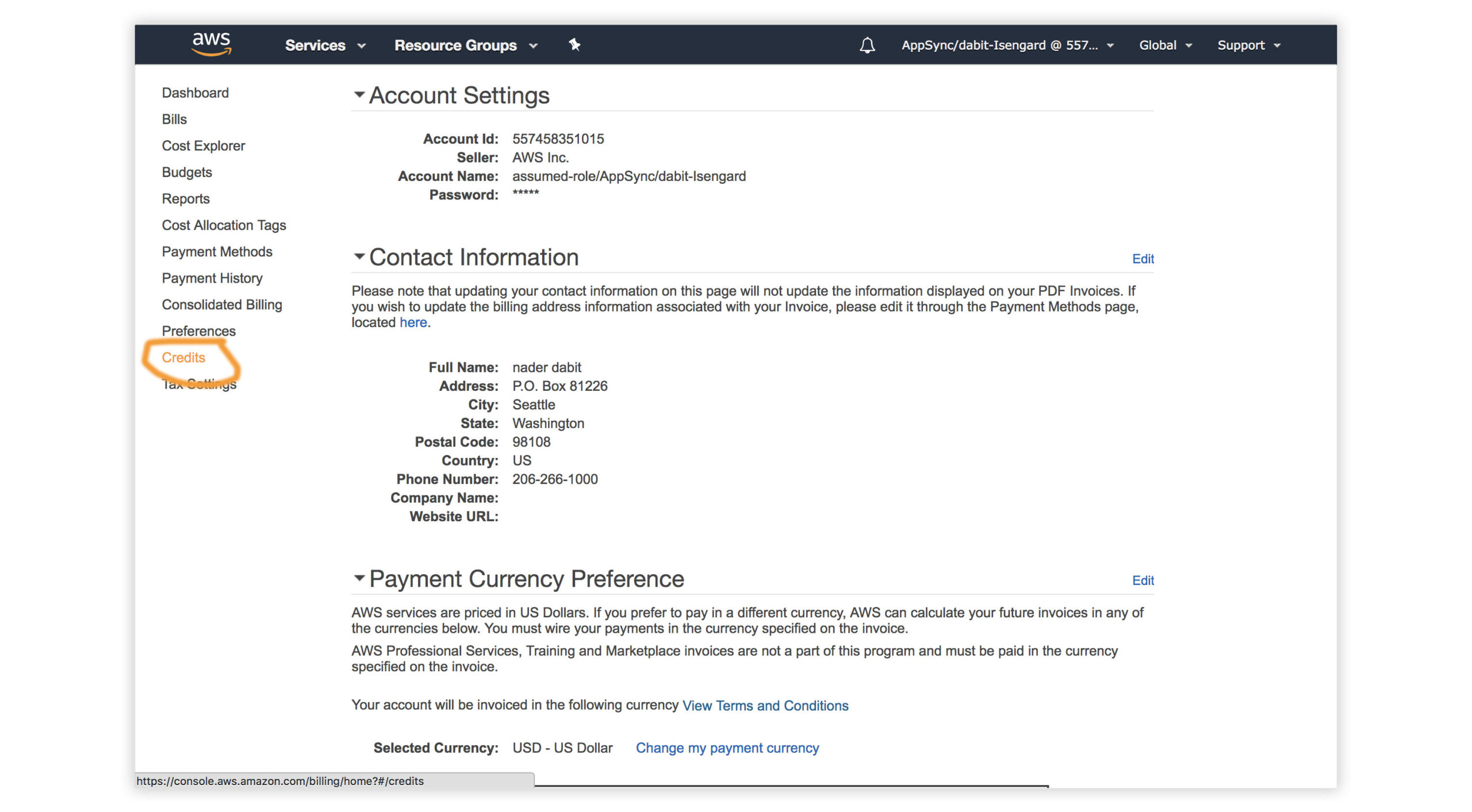
Here we’ll walk through the amplify configure setup. Once you’ve signed in to the AWS console, continue:
Specify the AWS Region: us-east-1 || us-west-2 || eu-central-1
Specify the username of the new IAM user: amplify-workshop-user
In the AWS Console, click Next: Permissions, Next: Tags, Next: Review, & Create User to create the new IAM user. Then, return to the command line & press Enter.
Enter the access key of the newly created user:
? accessKeyId: (<YOUR_ACCESS_KEY_ID>)
? secretAccessKey: (<YOUR_SECRET_ACCESS_KEY>)
Profile Name: amplify-workshop-user
Initializing A New Project
$ amplify init
Enter a name for the project: amplifyreactapp
Enter a name for the environment: dev
Choose your default editor: Visual Studio Code (or your default editor)
Please choose the type of app that you’re building javascript
What javascript framework are you using react
Source Directory Path: src
Distribution Directory Path: build
Build Command: npm run-script build
Start Command: npm run-script start
Do you want to use an AWS profile? Y
Please choose the profile you want to use: amplify-workshop-user
Now, the AWS Amplify CLI has iniatilized a new project & you will see a new folder: amplify & a new file called aws-exports.js in the src directory. These files hold your project configuration.
To view the status of the amplify project at any time, you can run the Amplify status command:
$ amplify status
Configuring the React applicaion
Now, our resources are created & we can start using them!
The first thing we need to do is to configure our React application to be aware of our new AWS Amplify project. We can do this by referencing the auto-generated aws-exports.js file that is now in our src folder.
To configure the app, open src/index.js and add the following code below the last import:
Now, our app is ready to start using our AWS services.
Adding a GraphQL API
To add a GraphQL API, we can use the following command:
$ amplify add api
? Please selectfrom one of the above mentioned services: GraphQL
? Provide API name: ConferenceAPI
? Choose an authorization typefor the API: API key
? Enter a description for the API key: <some description>? After how many days from now the API key should expire (1-365): 365
? Do you want to configure advanced settings for the GraphQL API: No
? Do you have an annotated GraphQL schema? N
? Do you want a guided schema creation? Y
? What best describes your project: Single object with fields
? Do you want to edit the schema now? (Y/n) Y
When prompted, update the schema to the following:
To mock and test the API locally, you can run the mock command:
$ amplify mock api

? Choose the code generation language target: javascript
? Enter the file name pattern of graphql queries, mutations and subscriptions: src/graphql/**/*.js
? Do you want to generate/update all possible GraphQL operations - queries, mutations and subscriptions: Y
? Enter maximum statement depth [increase from default if your schema is deeply nested]: 2
This should start an AppSync Mock endpoint:
AppSync Mock endpoint is running at http://10.219.99.136:20002
Open the endpoint in the browser to use the GraphiQL Editor.
From here, we can now test the API.
Performing mutations from within the local testing environment
Execute the following mutation to create a new talk in the API:
mutationcreateTalk {
createTalk(input: {
name: "Full Stack React"description: "Using React to build Full Stack Apps with GraphQL"speakerName: "Jennifer"speakerBio: "Software Engineer"
}) {
idnamedescriptionspeakerNamespeakerBio
}
}
Interacting with the GraphQL API from our client application – Querying for data
Now that the GraphQL API server is running we can begin interacting with it!
The first thing we’ll do is perform a query to fetch data from our API.
To do so, we need to define the query, execute the query, store the data in our state, then list the items in our UI.
src/App.js
// src/App.jsimportReactfrom'react';// imports from Amplify libraryimport{API,graphqlOperation}from'aws-amplify'// import query definitionimport{listTalksasListTalks}from'./graphql/queries'classAppextendsReact.Component{// define some state to hold the data returned from the APIstate={talks: []}// execute the query in componentDidMountasynccomponentDidMount(){try{consttalkData=awaitAPI.graphql(graphqlOperation(ListTalks))console.log('talkData:',talkData)this.setState({talks: talkData.data.listTalks.items})}catch(err){console.log('error fetching talks...',err)}}render(){return(<>{this.state.talks.map((talk,index)=>(<divkey={index}><h3>{talk.speakerName}</h3><h5>{talk.name}</h5><p>{talk.description}</p></div>))}</>)}}exportdefaultApp
In the above code we are using API.graphql to call the GraphQL API, and then taking the result from that API call and storing the data in our state. This should be the list of talks you created via the GraphiQL editor.
Feel free to add some styling here to your list if you’d like 😀
Next, test the app locally:
$ npm start
Performing mutations
Now, let’s look at how we can create mutations.
To do so, we’ll refactor our initial state in order to also hold our form fields and add an event handler.
We’ll also be using the API class from amplify again, but now will be passing a second argument to graphqlOperation in order to pass in variables: API.graphql(graphqlOperation(CreateTalk, { input: talk })).
We also have state to work with the form inputs, for name, description, speakerName, and speakerBio.
// src/App.jsimportReactfrom'react';import{API,graphqlOperation}from'aws-amplify'// import uuid to create a unique client IDimportuuidfrom'uuid/v4'import{listTalksasListTalks}from'./graphql/queries'// import the mutationimport{createTalkasCreateTalk}from'./graphql/mutations'constCLIENT_ID=uuid()classAppextendsReact.Component{// define some state to hold the data returned from the APIstate={name: '',description: '',speakerName: '',speakerBio: '',talks: []}// execute the query in componentDidMountasynccomponentDidMount(){try{consttalkData=awaitAPI.graphql(graphqlOperation(ListTalks))console.log('talkData:',talkData)this.setState({talks: talkData.data.listTalks.items})}catch(err){console.log('error fetching talks...',err)}}createTalk=async()=>{const{ name, description, speakerBio, speakerName }=this.stateif(name===''||description===''||speakerBio===''||speakerName==='')returnconsttalk={ name, description, speakerBio, speakerName,clientId: CLIENT_ID}consttalks=[...this.state.talks,talk]this.setState({
talks,name: '',description: '',speakerName: '',speakerBio: ''})try{awaitAPI.graphql(graphqlOperation(CreateTalk,{input: talk}))console.log('item created!')}catch(err){console.log('error creating talk...',err)}}onChange=(event)=>{this.setState({[event.target.name]: event.target.value})}render(){return(<><inputname='name'onChange={this.onChange}value={this.state.name}placeholder='name'/><inputname='description'onChange={this.onChange}value={this.state.description}placeholder='description'/><inputname='speakerName'onChange={this.onChange}value={this.state.speakerName}placeholder='speakerName'/><inputname='speakerBio'onChange={this.onChange}value={this.state.speakerBio}placeholder='speakerBio'/><buttononClick={this.createTalk}>Create Talk</button>{this.state.talks.map((talk,index)=>(<divkey={index}><h3>{talk.speakerName}</h3><h5>{talk.name}</h5><p>{talk.description}</p></div>))}</>)}}exportdefaultApp
Adding Authentication
Next, let’s update the app to add authentication.
To add authentication, we can use the following command:
$ amplify add auth

? Do you want to use default authentication and security configuration? Default configuration
? How do you want users to be able to sign in when using your Cognito User Pool? Username
? Do you want to configure advanced settings? No, I am done.
Using the withAuthenticator component
To add authentication in the React app, we’ll go into src/App.js and first import the withAuthenticator HOC (Higher Order Component) from aws-amplify-react:
// src/App.js, import the new componentimport{withAuthenticator}from'aws-amplify-react'
Next, we’ll wrap our default export (the App component) with the withAuthenticator HOC:
// src/App.js, change the default export to this:exportdefaultwithAuthenticator(App,{includeGreetings: true})
To deploy the authentication service and mock and test the app locally, you can run the mock command:
$ amplify mock

? Are you sure you want to continue? Yes
Next, to test it out in the browser:
npm start
Now, we can run the app and see that an Authentication flow has been added in front of our App component. This flow gives users the ability to sign up & sign in.
Accessing User Data
We can access the user’s info now that they are signed in by calling Auth.currentAuthenticatedUser() in componentDidMount.
import{API,graphqlOperation,/* new 👉 */Auth}from'aws-amplify'asynccomponentDidMount(){// add this code to componentDidMountconstuser=awaitAuth.currentAuthenticatedUser()console.log('user:',user)console.log('user info:',user.signInUserSession.idToken.payload)}
Adding Authorization to the GraphQL API
Next we need to update the AppSync API to now use the newly created Cognito Authentication service as the authentication type.
To do so, we’ll reconfigure the API:
$ amplify update api
? Please selectfrom one of the below mentioned services: GraphQL
? Choose the default authorization typefor the API: Amazon Cognito User Pool
? Do you want to configure advanced settings for the GraphQL API: No, I am done
Next, we’ll test out the API with authentication enabled:
$ amplify mock
Now, we can only access the API with a logged in user.
You’ll notice an auth button in the GraphiQL explorer that will allow you to update the simulated user and their groups.
Fine Grained access control – Using the @auth directive
GraphQL Type level authorization with the @auth directive
For authorization rules, we can start using the @auth directive.
What if you’d like to have a new Comment type that could only be updated or deleted by the creator of the Comment but can be read by anyone?
We could add the following type to our GraphQL schema:
Because we’re updating the way our database is configured by adding relationships which requires a global secondary index, we need to delete the old local database:
$ rm -r amplify/mock-data
Now, restart the server:
$ amplify mock
Now, we can create relationships between talks and comments. Let’s test this out with the following operations:
If you’d like to read more about the @auth directive, check out the documentation here.
Groups
The last problem we are facing is that anyone signed in can create a new talk. Let’s add authorization that only allows users that are in an Admin group to create and update talks.
Click on the auth button and add Admin the user’s groups.
Now, you’ll notice that only users in the Admin group can create, update, or delete a talk, but anyone can read it.
Lambda GraphQL Resolvers
Next, let’s have a look at how to deploy a serverless function and use it as a GraphQL resolver.
The use case we will work with is fetching data from another HTTP API and returning the response via GraphQL. To do this, we’ll use a serverless function.
The API we will be working with is the CoinLore API that will allow us to query for cryptocurrency data.
To get started, we’ll create the new function:
$ amplify add function
? Provide a friendly name foryour resource to be used as a label for this categoryin the project: currencyfunction
? Provide the AWS Lambda functionname: currencyfunction
? Choose the functiontemplate that you want to use: Hello world function
? Do you want to access other resources created in this project from your Lambda function? N
? Do you want to edit the local lambda functionnow? Y
In the above function we’ve used the axios library to call another API. In order to use axios, we need be sure that it will be installed by updating the package.json for the new function:
Next, we’ll update the GraphQL schema to add a new type and query. In amplify/backend/api/ConferenceAPI/schema.graphql, update the schema with the following new types:
This query should return an array of cryptocurrency information.
Deploying the Services
Next, let’s deploy the AppSync GraphQL API and the Lambda function:
$ amplify push

? Do you want to generate code for your newly created GraphQL API? Y
? Choose the code generation language target: javascript
? Enter the file name pattern of graphql queries, mutations and subscriptions: src/graphql/**/*.js
? Do you want to generate/update all possible GraphQL operations - queries, mutations and subscriptions? Y
? Enter maximum statement depth [increase from default if your schema is deeply nested] 2
To view the new AWS AppSync API at any time after its creation, run the following command:
$ amplify console api
To view the Cognito User Pool at any time after its creation, run the following command:
$ amplify console auth
To test an authenticated API out in the AWS AppSync console, it will ask for you to Login with User Pools. The form will ask you for a ClientId. This ClientId is located in src/aws-exports.js in the aws_user_pools_web_client_id field.
Hosting via the Amplify Console
The Amplify Console is a hosting service with continuous integration and continuous deployment.
The first thing we need to do is create a new GitHub repo for this project. Once we’ve created the repo, we’ll copy the URL for the project to the clipboard & initialize git in our local project:
Here, we’ll click on the app that we deployed earlier.
Next, under “Frontend environments”, authorize Github as the repository service.
Next, we’ll choose the new repository & branch for the project we just created & click Next.
In the next screen, we’ll create a new role & use this role to allow the Amplify Console to deploy these resources & click Next.
Finally, we can click Save and Deploy to deploy our application!
Now, we can push updates to Master to update our application.
Amplify DataStore
To implement a GraphQL API with Amplify DataStore, check out the tutorial here
Removing Services
If at any time, or at the end of this workshop, you would like to delete a service from your project & your account, you can do this by running the amplify remove command:
$ amplify remove auth

$ amplify push
If you are unsure of what services you have enabled at any time, you can run the amplify status command:
$ amplify status
amplify status will give you the list of resources that are currently enabled in your app.
If you’d like to delete the entire project, you can run the delete command:
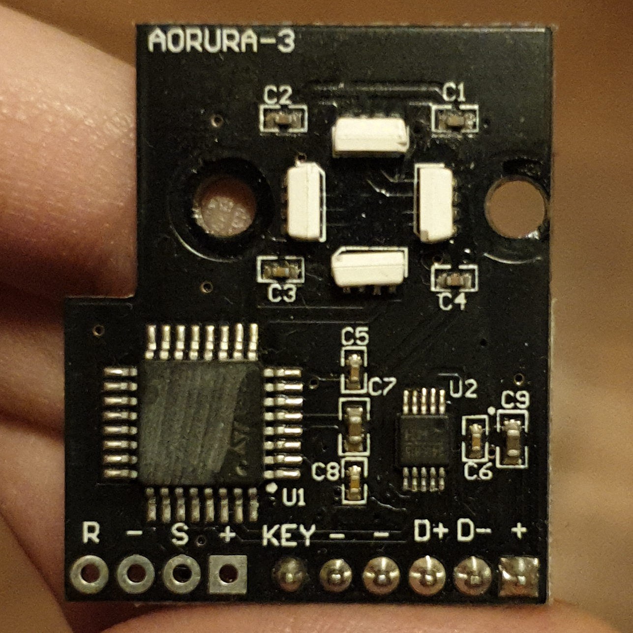
use aorura::*;use failure::*;fnmain() -> Fallible<()>{letmut led = Led::open("/dev/ttyUSB0")?;
led.set(State::Flash(Color::Red))?;
led.set(State::Off)?;assert_eq!(led.get()?,State::Off);assert_eq!(State::try_from(b"B*")?,State::Flash(Color::Blue));Ok(())}
Usage: aorura-cli <path> [--set STATE]
       aorura-cli --help

Gets/sets the AORURA LED state.

Options:
  --set STATE  set the LED to the given state

States: aurora, flash:COLOR, off, static:COLOR
Colors: blue, green, orange, purple, red, yellow
Example
path=/dev/ttyUSB0
original_state=$(aorura-cli $path)

aorura-cli $path --set flash:yellow

# Do something time-consuming:
sleep 10

# Revert back to the original LED state:
aorura-cli $path --set "$original_state"
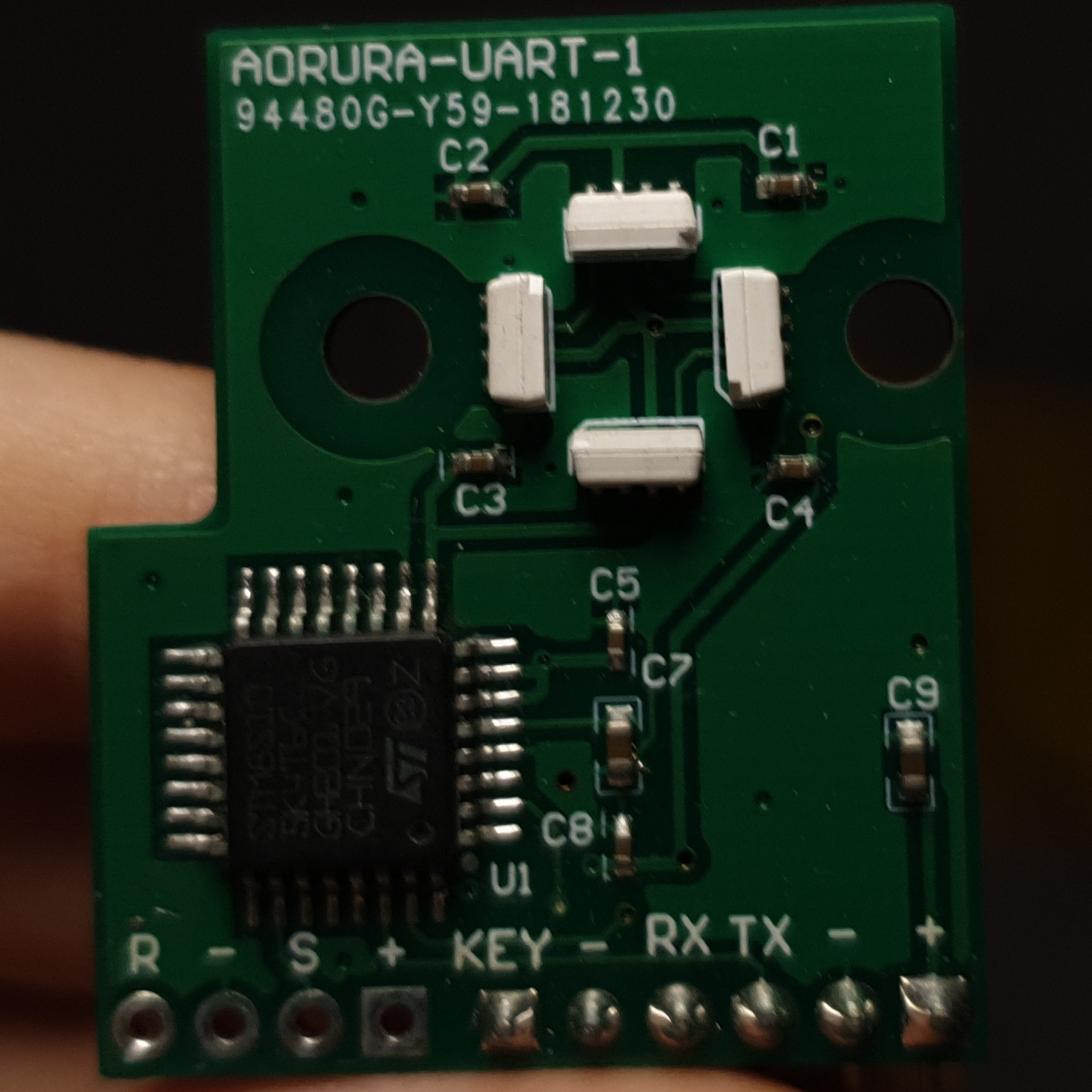
Emulator
aorura-emu is a PTY-based AORURA emulator. It can be used with
the library or the CLI in lieu of the hardware.
A Gymnasium environment for simulating and training reinforcement learning agents on the BlueROV2 underwater vehicle. This environment provides a realistic simulation of the BlueROV2’s dynamics and supports various control tasks.
🌊 Features
Realistic Physics: Implements validated hydrodynamic model of the BlueROV2
3D Visualization: Real-time 3D rendering using Meshcat
Custom Rewards: Configurable reward functions for different tasks
Disturbance Modeling: Includes environmental disturbances for realistic underwater conditions
Stable-Baselines3 Compatible: Ready to use with popular RL frameworks
Customizable Environment: Easy to modify for different underwater tasks
# Clone the repository
git clone https://github.com/gokulp01/bluerov2_gym.git
cd bluerov2_gym
# Create and activate a virtual environment
uv venv
source .venv/bin/activate # On Windows: .venv\Scripts\activate# Install the package
uv pip install -e .
Using pip
# Clone the repository
git clone https://github.com/gokulp01/bluerov2_gym.git
cd bluerov2_gym
# Create and activate a virtual environment
python -m venv .venv
source .venv/bin/activate # On Windows: .venv\Scripts\activate# Install the package
pip install -e .
🎮 Usage
Basic Usage
importgymnasiumasgymimportbluerov2_gym# Create the environmentenv=gym.make("BlueRov-v0", render_mode="human")
# Reset the environmentobservation, info=env.reset()
# Run a simple control loopwhileTrue:
# Take a random actionaction=env.action_space.sample()
observation, reward, terminated, truncated, info=env.step(action)
ifterminatedortruncated:
observation, info=env.reset()
Training with Stable-Baselines3 (refer to examples/train.py for full code example)
fromstable_baselines3importPPOfromstable_baselines3.common.vec_envimportDummyVecEnv, VecNormalize# Create and wrap the environmentenv=gym.make("BlueRov-v0")
env=DummyVecEnv([lambda: env])
env=VecNormalize(env)
# Initialize the agentmodel=PPO("MultiInputPolicy", env, verbose=1)
# Train the agentmodel.learn(total_timesteps=1_000_000)
# Save the trained modelmodel.save("bluerov_ppo")
🎯 Environment Details
State Space
The environment uses a Dictionary observation space containing:
x, y, z: Position coordinates
theta: Yaw angle
vx, vy, vz: Linear velocities
omega: Angular velocity
Action Space
Continuous action space with 4 dimensions:
Forward/Backward thrust
Left/Right thrust
Up/Down thrust
Yaw rotation
Reward Function
The default reward function considers:
Position error from target
Velocity penalties
Orientation error
Custom rewards can be implemented by extending the Reward class
📊 Examples
The examples directory contains several scripts demonstrating different uses:
test.py: Basic environment testing with manual control and evaluation with trained model
train.py: Training script using PPO
Running Examples
# Test environment with manual control
python examples/test.py

# Train an agent
python examples/train.py
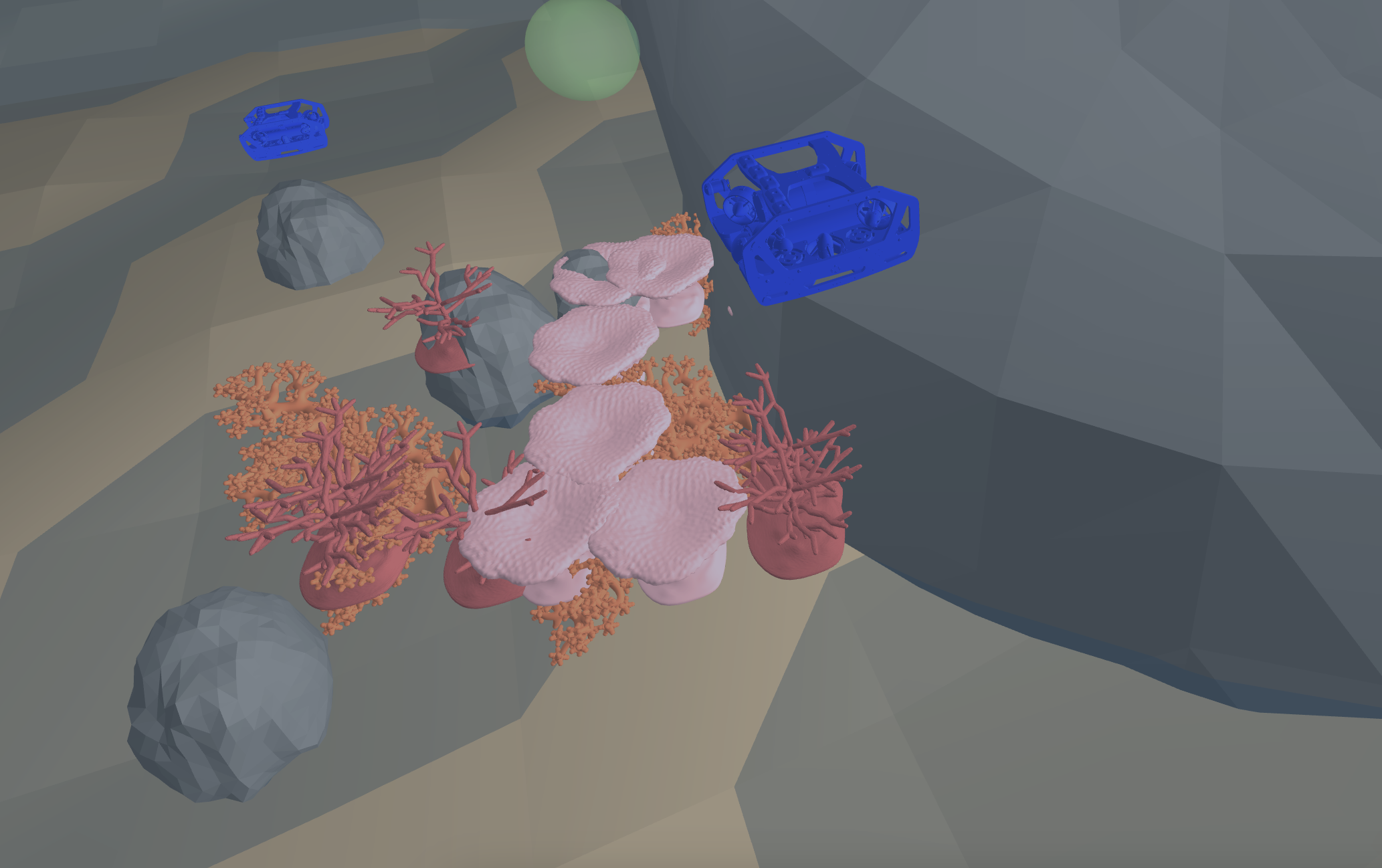
🖼️ Visualization
The environment uses Meshcat for 3D visualization. When running with render_mode="human", a web browser window will open automatically showing the simulation. The visualization includes:
Water surface effects
Underwater environment
ROV model
Ocean floor with decorative elements (I am no good at this)
📚 Project Structure
bluerov2_gym/
├── bluerov2_gym/              # Main package directory
│   ├── assets/               # 3D models and resources
│   └── envs/                 # Environment implementation
│       ├── core/            # Core components
│       │   ├── dynamics.py  # Physics simulation
│       │   ├── rewards.py   # Reward functions
│       │   ├── state.py     # State management
│       │   └── visualization/
│       │       └── renderer.py  # 3D visualization
│       └── bluerov_env.py    # Main environment class
├── examples/                  # Example scripts
├── tests/                    # Test cases
└── README.md
🔧 Configuration
The environment can be configured through various parameters:
Physics parameters in dynamics.py
Reward weights in rewards.py
Visualization settings in renderer.py
📝 Citation
If you use this environment in your research, please cite:
@article{puthumanaillam2024tabfieldsmaximumentropyframework,
title={TAB-Fields: A Maximum Entropy Framework for Mission-Aware Adversarial Planning},
author={Gokul Puthumanaillam and Jae Hyuk Song and Nurzhan Yesmagambet and Shinkyu Park and Melkior Ornik},
year={2024},
eprint={2412.02570},
archivePrefix={arXiv},
url={https://arxiv.org/abs/2412.02570} }}
🤝 Contributing
Contributions are welcome! Please feel free to submit a Pull Request. For major changes, please open an issue first to discuss what you would like to change.
Fork the repository
Create your feature branch (git checkout -b feature/AmazingFeature)
Commit your changes (git commit -m 'Add some AmazingFeature')
Push to the branch (git push origin feature/AmazingFeature)
Open a Pull Request
📄 License
This project is licensed under the MIT License
🙏 Acknowledgements
BlueRobotics for the BlueROV2 specifications
OpenAI/Farama Foundation for the Gymnasium framework
This tool helps convert Torch7 models into Apple CoreML format which can then be run on Apple devices.
Installation
pip install -U torch2coreml
In order to use this tool you need to have these installed:
Xcode 9
python 2.7
If you want to run tests, you need MacOS High Sierra 10.13 installed.
Dependencies
coremltools (0.6.2+)
PyTorch
How to use
Using this library you can implement converter for your own model types. An example of such a converter is located at “example/fast-neural-style/convert-fast-neural-style.py”.
To implement converters you should use single function “convert” from torch2coreml:
fromtorch2coremlimportconvert
This function is simple enough to be self-describing:
model: Torch7 model (loaded with PyTorch) | str
A trained Torch7 model loaded in python using PyTorch or path to file
with model (*.t7).
input_shapes: list of tuples
Shapes of the input tensors.
mode: str (‘classifier’, ‘regressor’ or None)
Mode of the converted coreml model:
‘classifier’, a NeuralNetworkClassifier spec will be constructed.
‘regressor’, a NeuralNetworkRegressor spec will be constructed.
deprocessing_args: dict
Same as ‘preprocessing_args’ but for deprocessing.
class_labels: A string or list of strings.
As a string it represents the name of the file which contains
the classification labels (one per line).
As a list of strings it represents a list of categories that map
the index of the output of a neural network to labels in a classifier.
predicted_feature_name: str
Name of the output feature for the class labels exposed in the Core ML
model (applies to classifiers only). Defaults to ‘classLabel’
unknown_layer_converter_fn: function with signature:
(builder, name, layer, input_names, output_names)
builder: object – instance of NeuralNetworkBuilder class
name: str – generated layer name
layer: object – PyTorch (python) object for corresponding layer
input_names: list of strings
output_names: list of strings
Returns: list of strings for layer output names
Callback function to handle unknown for torch2coreml layers
Returns
model: A coreml model.
Currently supported
Models
Only Torch7 “nn” module is supported now.
Layers
List of Torch7 layers that can be converted into their CoreML equivalent:
Sequential
ConcatTable
SpatialConvolution
ELU
ReLU
SpatialBatchNormalization
Identity
CAddTable
SpatialFullConvolution
SpatialSoftMax
SpatialMaxPooling
SpatialAveragePooling
View
Linear
Tanh
MulConstant
SpatialZeroPadding
SpatialReflectionPadding
Narrow
SpatialUpSamplingNearest
SplitTable
License
Copyright (c) 2017 Prisma Labs, Inc. All rights reserved.
Use of this source code is governed by the MIT License that can be found in the LICENSE.txt file.
Jovian is a Public Health toolkit to automatically process raw NGS data from human clinical matrices (faeces, serum, etc.) into clinically relevant information. It has three main components:
Illumina based Metagenomics:
Includes (amongst other features) data quality control, assembly, taxonomic classification, viral typing, and minority variant identification (quasispecies).
📝 Please refer to the documentation page for the Illumina Metagenomics workflow for more information.
Illumina based Reference-alignment:
Includes (amongst other features) data quality control, alignment, SNP identification, and consensus-sequence generation.
❗ A reference fasta is required.
📝 Please refer to the documentation page for the Illumina Reference based workflow for more information.
Nanopore based Reference-alignment:
Includes (amongst other features) data quality control, alignment, SNP identification, and consensus-sequence generation.
❗ A reference fasta is required.
❗ A fasta with primer sequences is required.
📝 Please refer to the documentation page for the Nanopore Reference based workflow for more information.
Key features of Jovian:
User-friendliness:
Wetlab personnel can start, configure and interpret results via an interactive web-report. Click here for an example report.
This makes doing Public Health analyses much more accessible and user-friendly since minimal command-line skills are required.
Audit trail:
All pipeline parameters, software versions, database information and runtime statistics are logged. See details below.
Portable:
Jovian is easily installed on off-site computer systems and at back-up sister institutes. Allowing results to be generated even when the internal grid-computer is down (speaking from experience).
Use case 3:
Align Nanopore (multiplex) PCR data against a user-provided reference, remove overrepresented primer sequences, and generate a consensus genome:
All cleaned reads are aligned against the user-provided reference fasta.
In the case of Nanopore (multiplex) PCR data, the overrepresented primer sequences are removed.
SNPs are called and a consensus genome is generated.
Consensus genomes are filtered at the following coverage cut-off thresholds: 1, 5, 10, 30 and 100x.
A tabular overview of the breadth of coverage (BoC) at the different coverage cut-off thresholds is generated.
Alignments and visualized via IGVjs and allow manual assessment and validation of consensus genomes.
Visualizations
All data are visualized via an interactive web-report, as shown here, which includes:
A collation of interactive QC graphs via MultiQC.
Taxonomic results are presented on three levels:
For an entire (multi sample) run, interactive heatmaps are made for non-phage viruses, phages and bacteria. They are stratified to different taxonomic levels.
For a sample level overview, Krona interactive taxonomic piecharts are generated.
For more detailed analyses, interactive tables are included. Similar to popular spreadsheet applications (e.g. Microsoft Excel).
Classified scaffolds
Unclassified scaffolds (i.e. “Dark Matter”)
Virus typing results are presented via interactive spreadsheet-like tables.
An interactive scaffold alignment viewer (IGVjs) is included, containing:
Detailed alignment information.
Depth of coverage graph.
GC content graph.
Predicted open reading frames (ORFs).
Identified minority variants (quasispecies).
All SNP metrics are presented via interactive spreadsheet-like tables, allowing detailed analysis.
Virus typing
After a Jovian analysis is finished you can perform virus-typing (i.e. sub-species level taxonomic labelling). These analyses can be started by the command bash jovian -vt [virus keyword], where [virus keyword] can be:
Keyword
Taxon used for scaffold selection
Notable virus species
NoV
Caliciviridae
Norovirus GI and GII, Sapovirus
EV
Picornaviridae
Enteroviruses (Coxsackie, Polio, Rhino, etc.), Parecho, Aichi, Hepatitis A
RVA
Rotavirus A
Rotavirus A
HAV
Hepatovirus A
Hepatitis A
HEV
Orthohepevirus A
Hepatitis E
PV
Papillomaviridae
Human Papillomavirus
Flavi
Flaviviridae
Dengue (work in progress)
all
All of the above
All of the above
Audit trail
An audit trail, used for clinical reproducibility and logging, is generated and contains:
A unique methodological fingerprint: allowing to exactly reproduce the analysis, even retrospectively by reverting to old versions of the pipeline code.
The following information is also logged:
Database timestamps
(user-specified) Pipeline parameters
However, it has limitations since several things are out-of-scope for Jovian to control:
The virus typing-tools version
Currently we depend on a public web-tool hosted by the RIVM. These are developed in close collaboration with – but independently of – Jovian. A versioning system for the virus typing-tools is being worked on, however, this is not trivial and will take some time.
Input files and metadata
We only save the names and location of input files at the time the analysis was performed. Long-term storage of the data, and documenting their location over time, is the responsibility of the end-user. Likewise, the end-user is responsible for storing datasets with their correct metadata (e.g. clinical information, database versions, etc.). We recommend using iRODS for this as described by Nieroda et al. 2019. While we acknowledge that database versions are vital to replicate results, the databases Jovian uses have no official versioning, hence why we include timestamps only.
Jovian Illumina Metagenomics workflow visualization
Click the image for a full-sized version
Jovian Illumina Reference alignment workflow visualization
Click the image for a full-sized version
Jovian Nanopore Reference alignment workflow visualization
Click the image for a full-sized version
Requirements
📝 Please refer to our documentation for a detailed overview of the Jovian requirements here
Installation
📝 Please refer to our documentation for detailed instructions regarding the installation of Jovian here
Usage instructions
General usage instructions vary for each workflow that we support.
Please refer to the link below corresponding to the workflow that you wish to use
Cock, P. J., Antao, T., Chang, J. T., Chapman, B. A., Cox, C. J., Dalke, A., … & De Hoon, M. J. (2009). Biopython: freely available Python tools for computational molecular biology and bioinformatics. Bioinformatics, 25(11), 1422-1423.
Wilm, A., et al., LoFreq: a sequence-quality aware, ultra-sensitive variant caller for uncovering cell-population heterogeneity from high-throughput sequencing datasets. 2012. 40(22): p. 11189-11201.
Rubino, F. and Creevey, C.J. 2014. MGkit: Metagenomic Framework For The Study Of Microbial Communities. . Available at: figshare [doi:10.6084/m9.figshare.1269288].
Walt, S. V. D., Colbert, S. C., & Varoquaux, G. (2011). The NumPy array: a structure for efficient numerical computation. Computing in Science & Engineering, 13(2), 22-30.
Kroneman, A., Vennema, H., Deforche, K., Avoort, H. V. D., Penaranda, S., Oberste, M. S., … & Koopmans, M. (2011). An automated genotyping tool for enteroviruses and noroviruses. Journal of Clinical Virology, 51(2), 121-125.
This project/research has received funding from the European Union’s Horizon 2020 research and innovation programme under grant agreement No. 643476. and the Dutch working group on molecular diagnostics (WMDI).